library(tidyverse)

theme_set(theme_minimal())

atp_df <- read_csv("https://raw.githubusercontent.com/JeffSackmann/tennis_atp/master/atp_matches_2024.csv") |>
  mutate(tour = "atp")
wta_df <- read_csv("https://raw.githubusercontent.com/JeffSackmann/tennis_wta/master/wta_matches_2024.csv") |>
  mutate(tour = "wta")

both_df <- bind_rows(atp_df, wta_df)

both_long <- both_df |> pivot_longer(c(winner_name, loser_name))

## only keep players who have player over 50 matches
both_n50 <- both_long |> group_by(value) |> summarise(n = n()) |>
  filter(n > 50)

## construct various statistics
major_tennis <- semi_join(both_long, both_n50, by = c("value"))
major_tennis <- major_tennis |> mutate(w_svperc = 100 * w_1stIn / w_svpt,
                        l_svperc = 100 * l_1stIn / l_svpt,
                        w_firstwon = 100 * w_1stWon / w_1stIn,
                        l_firstwon = 100 * l_1stWon / l_1stIn,
                        w_secondwon = 100 * w_2ndWon / (w_svpt - w_1stIn),
l_secondwon = 100 * l_2ndWon / (l_svpt - l_1stIn))15 Shiny Reactivity
Working with shiny can be difficult at first because we need to think about how code is run a bit differently. In .rmd, .qmd, and .R files, code is run from beginning to end. This makes debugging relatively simple: we run code line by line until we get an error. Then, we try to understand why the code gives an error.
On the other hand, code in a shiny app does not run from beginning to end. Instead, code is run through a process called reactive execution. We will explore this concept by making reactive graphs. We will begin this section with a reading from the Mastering Shiny book and then delve into more examples.
15.1 Basic Reactivity (Class Prep)
Read Sections 3.1 through 3.3 in the Basic Reactivity Chapter of Mastering Shiny
Exercise 1. 3.3.6 Exercise 1 in Mastering Shiny.
Exercise 2. 3.3.6 Exercise 2 in Mastering Shiny. You do not need to submit your sketches but you should bring them to class.
15.2 Another Example Tennis App
The purpose of this section is to complete another example with a different data set, continuing to strengthen our conceptual understanding of reactivity. We will use a couple of tennis data sets obtained from https://github.com/JeffSackmann/tennis_atp and https://github.com/JeffSackmann/tennis_wta to create an app that lets us create a histogram of a summary statistic of our choosing for a player of our choosing. Constructing this app will cover another common use case: allowing a user to choose a variable from a data set to plot.
Again, a usual first step is creating a static graph, choosing a value for each future interactive input. Begin by reading in the data and doing a bit of preparatory work. To focus on shiny, we will skip discussion of this work, but all of it are functions you should recognize.
The next chunk of code is needed to put the various statistics into one column. This is an issue because, in major_tennis, there is a column for w_ace (aces for the winner) and l_ace (aces for the loser). We need those in one column, aces, that have the number of aces for the player. Looking back, this is not the most efficient way we could do this. If we were to do it again, we could do an across() combined with if_else() where the new variables would take the w_.... values if the player was the winner and the l_.... values if the player was the loser.
major_tennis_w <- major_tennis |> filter(name == "winner_name")
major_tennis_l <- major_tennis |> filter(name == "loser_name")

w_small <- major_tennis_w |> select(value, winner_seed, w_ace, w_df,
                                    w_svperc, w_firstwon, w_secondwon,
                                    tour) |>
  rename(seed = winner_seed, ace = w_ace, df = w_df, svperc = w_svperc,
         firstwon = w_firstwon, secondwon = w_secondwon)

l_small <- major_tennis_l |> select(value, loser_seed, l_ace, l_df,
                                    l_svperc, l_firstwon, l_secondwon,
                                    tour) |>
  rename(seed = loser_seed, ace = l_ace, df = l_df, svperc = l_svperc,
         firstwon = l_firstwon, secondwon = l_secondwon)

df <- bind_rows(w_small, l_small) |>
  rename(player = "value")
df
#> # A tibble: 3,985 × 8
#>   player           seed   ace    df svperc firstwon secondwon tour
#>   <chr>           <dbl> <dbl> <dbl>  <dbl>    <dbl>     <dbl> <chr>
#> 1 Grigor Dimitrov     2     8     2   70.3     76.9      59.1 atp
#> 2 Holger Rune         1     7     4   66.7     81.2      45.8 atp
#> 3 Grigor Dimitrov     2    10     3   67.2     86.7      45.5 atp
#> 4 Holger Rune         1    13     0   55.4     86.1      58.6 atp
#> 5 Jordan Thompson    NA     8     3   61.5     76.1      47.6 atp
#> 6 Grigor Dimitrov     2    12     2   66       78.8      70.6 atp
#> # ℹ 3,979 more rows
Now, we have our five variables (ace, df, svperc, firstwon, and secondwon). We want an app that lets that user make a histogram of one of these variables for a player of their choosing.
We will try to use a similar workflow for this problem as we did for the majors app.
Step 1: Make a histogram of one variable for one specific player.
Step 2: Set up our shiny app inputs. Before, we just had a single input. Now, we will have two: one for player and one for variable. Let’s focus on one at a time, doing player first. Type shinyapp and click on the R Studio snippet to bring up a base app. Then, add player as an input in sidebarPanel() part of a sidebarLayout() UI.
Step 3: Now that we have one of our inputs in the UI, let’s work on the server. First, we will ignore the input$ selector and put in our graph from step 1. We again use the plotOutput(), renderPlot({}) combination.
Step 4: Now we want to connect the input defined in the UI to the server so that the graph changes depending on which player we select.
Step 5: We can then repeat some of these steps for a second input: a variable that the user selects. We will use radioButtons() as the input in the UI.
We will discuss why we need to take some extra steps to perform the “user can select a variable” operation in class. In particular, we will need to briefly discuss tidy evaluation to use some of the tidyverse functions in shiny (see Section 15.4.1).
Step 6: Add a third input that will let the user change the number of bins in the histogram.
Step 7: Use the glue() function from the glue package to change the title of the histogram to include the name of the player in the plot (see Section 15.4.2).
Step 8: Suppose that we want to add a buttons that the user can select corresponding to the two main professional tennis tours (atp for the men’s tour and wta for the women’s tour). After the user selects an appropriate tour, we want the player choices to give players corresponding only to that tour (so that only men appear when atp is selected and only women appear when wta is selected). To make something like this happen, we need to learn about how to make the UI dynamic (Section 15.4.3).
Exercise 1. If we move the output$name_of_histogram <- .... code to the very beginning of the server function, do you think the app will still run? Give a reason.
Exercise 2. Draw the reactive graph for the Tennis app. Make sure to include all inputs, outputs, and reactive expressions in your graph.
Exercise 3. Sketch the reactive graph for the majors app in the previous section. Make sure to include all inputs, outputs, and reactive expressions in your graph.
15.3 Your Turn
Exercise 1. In the tennis app, change the histogram input from a sliderInput() to a numericInput().
Exercise 2. In the tennis app, change the histogram input back to sliderinput(). Then, apply 2.2.8 Exercise 3 in the Mastering Shiny book to the tennis app slider.
Exercise 3. Add an additional input or output (or both!) to the Tennis App. You can decide what you want to add here!
Exercise 4. The following app UI was taken from the Mastering Shiny book. With the app skeleton, complete the following.
library(shiny)
library(gapminder)
continents <- unique(gapminder$continent)

ui <- fluidPage(
  selectInput("continent", "Continent", choices = continents),
  selectInput("country", "Country", choices = NULL),
  tableOutput("data")
)

server <- function(input, output, session) {

}
Complete the server function so that the country choices update according to the continent that the user selects. Have the app display a table with the corresponding rows to the country that the user then selects.
Add an action button so that the table only updates after the user clicks the button (see Section 15.4.4).
Extend the app so that there is an option to choose “All” for continent, which lets you see all of the countries in the list. To do this, you can use a base
Rif elsestatement (see Section 15.4.5) to trigger the “special” case for when “All” is selected. You can also use this code to get “All” to appear as an option in your list of choices for the continent:
continents <- continents |> fct_expand("All")
15.4 Other Useful Things for shiny
15.4.1 Tidy Evaluation
When using some tidyverse functions inside of a function environment, there are some issues in that we are mixing two different types of “variables” in R. In particular,
- an environmental variable is something created using
<-. Theinput$name_of_varare environmental variables. - a data variable is a variable that is inside of a data frame.
The same issues encountered with tidy evaluation in shiny are also encountered in more generic functions. Let’s examine this issue in functions first, as it’s a little bit quicker to see what’s happening (as opposed to shiny, where we have to run the entire app). But, keep in mind that the server part of shiny is a function itself, so we will have all of these same issues.
The following are some toy functions performing various tasks on the mtcars data. Which ones work how you expect? Which ones do not?
subset_by_cyl <- function(cyl_val) {
  mtcars |> filter(cyl == cyl_val)
}
subset_by_cyl(cyl_val = 8)
#>                      mpg cyl  disp  hp drat    wt  qsec vs am gear carb
#> Hornet Sportabout   18.7   8 360.0 175 3.15 3.440 17.02  0  0    3    2
#> Duster 360          14.3   8 360.0 245 3.21 3.570 15.84  0  0    3    4
#> Merc 450SE          16.4   8 275.8 180 3.07 4.070 17.40  0  0    3    3
#> Merc 450SL          17.3   8 275.8 180 3.07 3.730 17.60  0  0    3    3
#> Merc 450SLC         15.2   8 275.8 180 3.07 3.780 18.00  0  0    3    3
#> Cadillac Fleetwood  10.4   8 472.0 205 2.93 5.250 17.98  0  0    3    4
#> Lincoln Continental 10.4   8 460.0 215 3.00 5.424 17.82  0  0    3    4
#> Chrysler Imperial   14.7   8 440.0 230 3.23 5.345 17.42  0  0    3    4
#> Dodge Challenger    15.5   8 318.0 150 2.76 3.520 16.87  0  0    3    2
#> AMC Javelin         15.2   8 304.0 150 3.15 3.435 17.30  0  0    3    2
#> Camaro Z28          13.3   8 350.0 245 3.73 3.840 15.41  0  0    3    4
#> Pontiac Firebird    19.2   8 400.0 175 3.08 3.845 17.05  0  0    3    2
#> Ford Pantera L      15.8   8 351.0 264 4.22 3.170 14.50  0  1    5    4
#> Maserati Bora       15.0   8 301.0 335 3.54 3.570 14.60  0  1    5    8
subset_by_cyl(cyl_val = "8")
#>                      mpg cyl  disp  hp drat    wt  qsec vs am gear carb
#> Hornet Sportabout   18.7   8 360.0 175 3.15 3.440 17.02  0  0    3    2
#> Duster 360          14.3   8 360.0 245 3.21 3.570 15.84  0  0    3    4
#> Merc 450SE          16.4   8 275.8 180 3.07 4.070 17.40  0  0    3    3
#> Merc 450SL          17.3   8 275.8 180 3.07 3.730 17.60  0  0    3    3
#> Merc 450SLC         15.2   8 275.8 180 3.07 3.780 18.00  0  0    3    3
#> Cadillac Fleetwood  10.4   8 472.0 205 2.93 5.250 17.98  0  0    3    4
#> Lincoln Continental 10.4   8 460.0 215 3.00 5.424 17.82  0  0    3    4
#> Chrysler Imperial   14.7   8 440.0 230 3.23 5.345 17.42  0  0    3    4
#> Dodge Challenger    15.5   8 318.0 150 2.76 3.520 16.87  0  0    3    2
#> AMC Javelin         15.2   8 304.0 150 3.15 3.435 17.30  0  0    3    2
#> Camaro Z28          13.3   8 350.0 245 3.73 3.840 15.41  0  0    3    4
#> Pontiac Firebird    19.2   8 400.0 175 3.08 3.845 17.05  0  0    3    2
#> Ford Pantera L      15.8   8 351.0 264 4.22 3.170 14.50  0  1    5    4
#> Maserati Bora       15.0   8 301.0 335 3.54 3.570 14.60  0  1    5    8

plot_mtscatter <- function(x_var, y_var) {
  ggplot(data = mtcars, aes(x = x_var, y = y_var)) +
    geom_point() +
    theme_minimal()
}

plot_mtscatter(x_var = "hp", y_var = "mpg")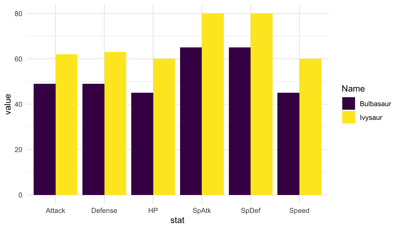
sort_mtcars <- function(var_sort) {
  mtcars |> arrange(var_sort)
}
sort_mtcars(var_sort = "mpg")
#>                      mpg cyl  disp  hp drat    wt  qsec vs am gear carb
#> Mazda RX4           21.0   6 160.0 110 3.90 2.620 16.46  0  1    4    4
#> Mazda RX4 Wag       21.0   6 160.0 110 3.90 2.875 17.02  0  1    4    4
#> Datsun 710          22.8   4 108.0  93 3.85 2.320 18.61  1  1    4    1
#> Hornet 4 Drive      21.4   6 258.0 110 3.08 3.215 19.44  1  0    3    1
#> Hornet Sportabout   18.7   8 360.0 175 3.15 3.440 17.02  0  0    3    2
#> Valiant             18.1   6 225.0 105 2.76 3.460 20.22  1  0    3    1
#> Duster 360          14.3   8 360.0 245 3.21 3.570 15.84  0  0    3    4
#> Merc 240D           24.4   4 146.7  62 3.69 3.190 20.00  1  0    4    2
#> Merc 230            22.8   4 140.8  95 3.92 3.150 22.90  1  0    4    2
#> Merc 280            19.2   6 167.6 123 3.92 3.440 18.30  1  0    4    4
#> Merc 280C           17.8   6 167.6 123 3.92 3.440 18.90  1  0    4    4
#> Merc 450SE          16.4   8 275.8 180 3.07 4.070 17.40  0  0    3    3
#> Merc 450SL          17.3   8 275.8 180 3.07 3.730 17.60  0  0    3    3
#> Merc 450SLC         15.2   8 275.8 180 3.07 3.780 18.00  0  0    3    3
#> Cadillac Fleetwood  10.4   8 472.0 205 2.93 5.250 17.98  0  0    3    4
#> Lincoln Continental 10.4   8 460.0 215 3.00 5.424 17.82  0  0    3    4
#> Chrysler Imperial   14.7   8 440.0 230 3.23 5.345 17.42  0  0    3    4
#> Fiat 128            32.4   4  78.7  66 4.08 2.200 19.47  1  1    4    1
#> Honda Civic         30.4   4  75.7  52 4.93 1.615 18.52  1  1    4    2
#> Toyota Corolla      33.9   4  71.1  65 4.22 1.835 19.90  1  1    4    1
#> Toyota Corona       21.5   4 120.1  97 3.70 2.465 20.01  1  0    3    1
#> Dodge Challenger    15.5   8 318.0 150 2.76 3.520 16.87  0  0    3    2
#> AMC Javelin         15.2   8 304.0 150 3.15 3.435 17.30  0  0    3    2
#> Camaro Z28          13.3   8 350.0 245 3.73 3.840 15.41  0  0    3    4
#> Pontiac Firebird    19.2   8 400.0 175 3.08 3.845 17.05  0  0    3    2
#> Fiat X1-9           27.3   4  79.0  66 4.08 1.935 18.90  1  1    4    1
#> Porsche 914-2       26.0   4 120.3  91 4.43 2.140 16.70  0  1    5    2
#> Lotus Europa        30.4   4  95.1 113 3.77 1.513 16.90  1  1    5    2
#> Ford Pantera L      15.8   8 351.0 264 4.22 3.170 14.50  0  1    5    4
#> Ferrari Dino        19.7   6 145.0 175 3.62 2.770 15.50  0  1    5    6
#> Maserati Bora       15.0   8 301.0 335 3.54 3.570 14.60  0  1    5    8
#> Volvo 142E          21.4   4 121.0 109 4.11 2.780 18.60  1  1    4    2

select_mtcars <- function(var_select) {
  mtcars |> select(var_select)
}
select_mtcars(var_select = "mpg")
#>                      mpg
#> Mazda RX4           21.0
#> Mazda RX4 Wag       21.0
#> Datsun 710          22.8
#> Hornet 4 Drive      21.4
#> Hornet Sportabout   18.7
#> Valiant             18.1
#> Duster 360          14.3
#> Merc 240D           24.4
#> Merc 230            22.8
#> Merc 280            19.2
#> Merc 280C           17.8
#> Merc 450SE          16.4
#> Merc 450SL          17.3
#> Merc 450SLC         15.2
#> Cadillac Fleetwood  10.4
#> Lincoln Continental 10.4
#> Chrysler Imperial   14.7
#> Fiat 128            32.4
#> Honda Civic         30.4
#> Toyota Corolla      33.9
#> Toyota Corona       21.5
#> Dodge Challenger    15.5
#> AMC Javelin         15.2
#> Camaro Z28          13.3
#> Pontiac Firebird    19.2
#> Fiat X1-9           27.3
#> Porsche 914-2       26.0
#> Lotus Europa        30.4
#> Ford Pantera L      15.8
#> Ferrari Dino        19.7
#> Maserati Bora       15.0
#> Volvo 142E          21.4
We will spend a little time fixing the code that does not work.
15.4.2 glue::glue()
The glue() function from the glue package is really useful for making plot titles, axis titles, etc. that depend on variables you have made. For example, you might want a title for ggplot2 to change depending on which input a user selects.
It’s a fairly simple function: you just put together text in " " and variable names, separated by commas.
poke_df <- read_csv(here::here("data/pokemon_full.csv"))
poke_long <- poke_df |> pivot_longer(4:9, values_to = "value",
                                      names_to = "stat")

library(shiny)

ui <- fluidPage(
  sidebarLayout(
    sidebarPanel(
      selectizeInput("pokechoose1", label = "Choose Pokemon",
                     choices = poke_df$Name, selected = "Bulbasaur")
    ),
    mainPanel(
      plotOutput(outputId = "pokegraph")
    )
  )
)

server <- function(input, output, session) {

  output$pokegraph <- renderPlot({
    poke_react <- poke_long |> filter(Name %in% input$pokechoose1)

    ggplot(data = poke_react, aes(x = stat, y = value)) +
      geom_point() +
      geom_segment(aes(xend = stat, y = 0, yend = value)) +
      coord_flip() +
      labs(title = glue::glue("Graph of the Stats for", input$pokechoose1))
  })

}

shinyApp(ui, server)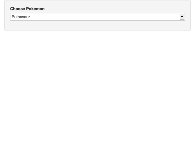
15.4.3 Dynamic UI
For what we have learned about so far, we have set up a Shiny app so that, when the user changes something in the user interface (UI), something else in the server changes. But suppose that we would the UI itself to update when the user changes something in the UI. If we want the UI to update based on what a user selects, then we want the UI to be dynamic.
As an example, suppose that in the previous Pokemon example, we want the user to choose a pokemon Generation (1, 2, 3, 4, 5, 6) and to have our list only contain Pokemon for that particular Generation. This situation calls for dynamic UI because our selectizeInput UI component should update when the user chooses a Generation in the UI.
poke_df <- read_csv(here::here("data/pokemon_full.csv"))
poke_long <- poke_df |> pivot_longer(4:9, values_to = "value",
                                      names_to = "stat")

library(shiny)

ui <- fluidPage(
  sidebarLayout(
    sidebarPanel(
      selectInput("genchoose", label = "Choose a Generation",
                  choices = 1:6, selected = 1),
      selectizeInput("pokechoose1", label = "Choose Pokemon",
                     choices = poke_df$Name, selected = "Bulbasaur")
    ),
    mainPanel(
      plotOutput(outputId = "pokegraph")
    )
  )
)

server <- function(input, output, session) {

  observeEvent(input$genchoose, {
    pokemon_choices <- poke_df |>
      filter(Generation == input$genchoose) |>
      pull(Name) ## makes the Name a vector
    updateSelectizeInput(inputId = "pokechoose1", choices = pokemon_choices)
  })

  output$pokegraph <- renderPlot({
    poke_react <- poke_long |> filter(Name %in% input$pokechoose1)

    ggplot(data = poke_react, aes(x = stat, y = value)) +
      geom_point() +
      geom_segment(aes(xend = stat, y = 0, yend = value)) +
      coord_flip() +
      labs(title = glue::glue("Graph of the Stats for", input$pokechoose1))
  })

}

shinyApp(ui, server)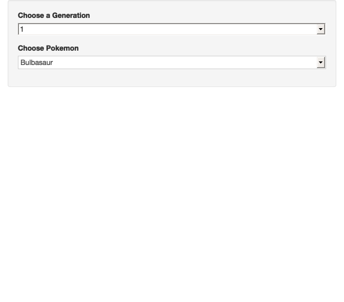
In the code above, there are a few new pieces we added to get the UI to update dynamically:
- we added a
selectInputpiece in the UI so that a user can select aGeneration. - we added an
observeEventpiece in the server. The first argument ofobserveEventgives the event that we want shiny to “watch for”. In this case, the event that we are watching for is a change to the “choose generation” input. - when
input$genchooseis changed by the user, Shiny “observes this event,” which triggers the code in the{}to run. - the code within the
{}filters the pokemon data set according to theGenerationselected and puts all of the pokemonNames from thisGenerationinto a vector. - finally, the
updateSelectizeInputpiece tells theselectizeInputin the UI to update with these new choices.
15.4.5 Using if and else
If we want our app do do something completely different when a user changes an input, we might consider using if and else. If we have time in class, we will do an example in Shiny: if an input is equal to some value, do something or make a certain plot; else make a different type of plot. Below is an example of the syntax in base R:
x <- 5
if (x < 10) {
  x * 2
} else {
  x / 2
}
#> [1] 10
15.4.6 source() and write_csv()
ImportantImportant
For shiny apps, if there is a lot of data preparation before the data is ready for the shiny app, it is generally best to put this data preparation in a different R script.
You can then either source() the data preparation file (which runs all of the code in the file that is sourced) or you can use write_csv() to write the prepped data to its own .csv file. You would then use read_csv() on this new file in the app.R file with your shiny app.