run a permutation test on a couple of different data sets to assess two competing hypotheses.
use empirical power to compute the approximate power of a test under a few different assumptions.
Lab 5.1: Permutation Tests
In this lab, we use permutation tests to assess whether there is evidence that the mean delay times of two different airlines are different and whether there is evidence that completing a difficult task with a dog in the room lowers stress level, on average.
Example 1: Flight Data
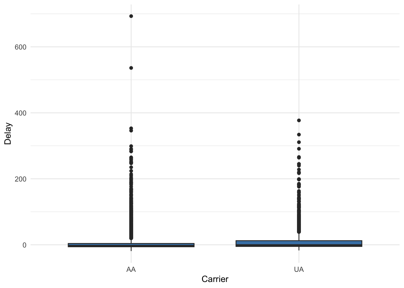
Consider again the flight delay data. Here, we will consider whether or not there is statistical evidence that the mean delay of United Airlines is different than the mean delay of American Airlines.
Recall that, for a permutation test, we do not need to assume that the underlying populations follow a normal distribution. However, if we are interested in testing a difference in means, we do need to assume that the populations have the same variance and the same shape (but perhaps may have a different center). Note that, if we have a randomized experiment, then these assumptions can be relaxed.
First, we obtain some summary statistics and make a plot of the data:
We next store the difference in sample means as a value called teststat and each of the sample sizes as n_a and n_u:
teststat<-delay_df|>group_by(Carrier)|>summarise(mean_delay =mean(Delay))|>pull(mean_delay)|>diff()## teststat is united delay mean minus american airlines mean
Under the null hypothesis, the distribution of delays is identical for american and united airlines. To reshuffle the delay values randomly across both airlines we can use the code below:
# A tibble: 4,029 × 11
   delay_perm Carrier Delay    ID FlightNo Destination DepartTime Day   Month
        <int> <fct>   <int> <int>    <int> <fct>       <fct>      <fct> <fct>
 1         -4 UA         -1     1      403 DEN         4-8am      Fri   May
 2         -6 UA        102     2      405 DEN         8-Noon     Fri   May
 3         -2 UA          4     3      409 DEN         4-8pm      Fri   May
 4          0 UA         -2     4      511 ORD         8-Noon     Fri   May
 5         87 UA         -3     5      667 ORD         4-8am      Fri   May
 6        120 UA          0     6      669 ORD         4-8am      Fri   May
 7         -9 UA         -5     7      673 ORD         8-Noon     Fri   May
 8         -3 UA          0     8      677 ORD         8-Noon     Fri   May
 9         -6 UA         10     9      679 ORD         Noon-4pm   Fri   May
10          6 UA         60    10      681 ORD         Noon-4pm   Fri   May
# ℹ 4,019 more rows
# ℹ 2 more variables: FlightLength <int>, Delayed30 <fct>
Rerun the previous code chunk a few times to see a different permutations of the Delay variable.
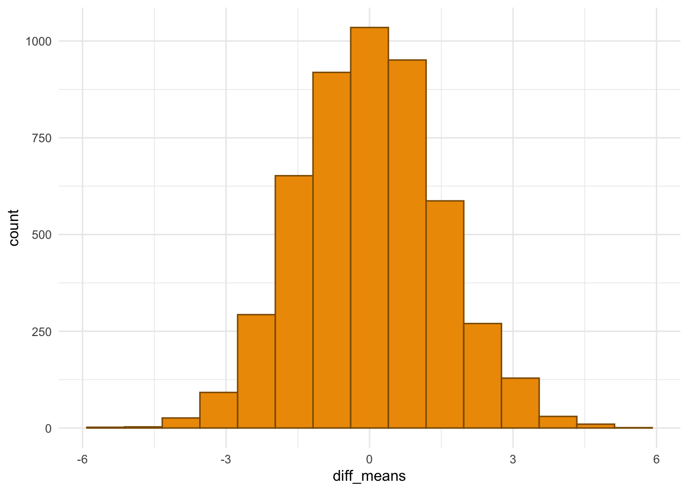
With one permutation, we want to recalculate the difference in means:
Rerun the code chunk above a few times to get a few different mean differences under different permutations. The big idea is that a large number of these mean differences will form the null distribution for the difference in sample means (if there really is no difference in the underlying population distributions).
So, let’s wrap that above code in a function, and then iterate over that function a large number of times to obtain our null distribution:
Exercise. Before explicitly calculating a p-value, assess visually whether a p-value for this hypothesis test will be relatively large or relatively small.
Now, let’s explicitly compute a conservative p-value for the test:
Exercise. What is the alternative hypothesis that the p-value is testing?
Exercise. What is the purpose of the + 1 in the code above?
Exercise. Why are there two different summations in the code above to get the p-value?
Exercise. Write a conclusion in context of the problem for this hypothesis test.
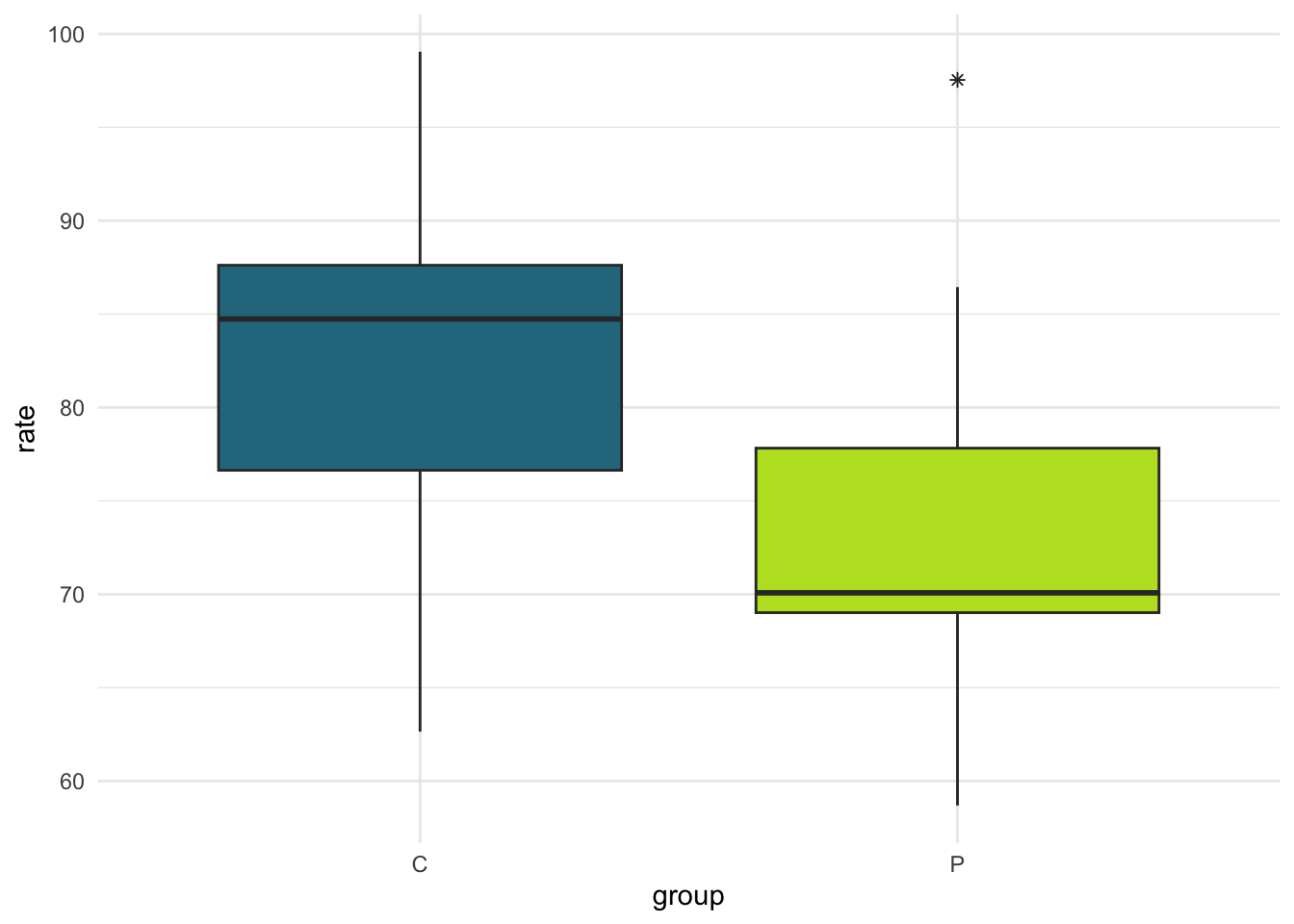
Example 2: Stress Levels
Many of you took our probability exams with the adorable Mipha providing moral support throughout the exam. There has actually been formal research assessing whether being in the presence of a dog can have beneficial effects for people. In one such study, researchers recruited 30 women who were self-proclaimed dog lovers. They randomly assigned 15 women to a stressful task alone (control: C) and 15 women to do a stressful task with a pet dog present (pet: P). The response variable is heart rate during the task, with higher heart rates presumed to mean that the there was more stress during the task.
Use the code below to read in the data and do some brief data exploration:
Rows: 30 Columns: 2
── Column specification ────────────────────────────────────────────────────────
Delimiter: ","
chr (1): group
dbl (1): rate

ℹ Use `spec()` to retrieve the full column specification for this data.
ℹ Specify the column types or set `show_col_types = FALSE` to quiet this message.
Exercise. Write a conclusion in context of the problem for this hypothesis test.
Lab 5.2: Asymptotic LRTs in Practice
In this lab, we will see an example of how an asymptotic likelihood ratio test is used in practice.
Logistic Regression Example
If you took STAT 213, recall the logistic regression model that you used in that course:
\(Y_i \sim \text{Bernoulli}(p_i)\), where each \(Y_i\) is independent of all other \(Y_j\) but the \(Y_i\) are not identically distributed. Instead, each \(Y_i\) is allowed to have its own probability of success, \(p_i\), which can be modeled as:
Cumings, Mrs. John Bradley (Florence Briggs Thayer)
female
38
1
3rd
Heikkinen, Miss. Laina
female
26
Exercise. Suppose that we want to build a logistic regression model with Survived (a 1 is survived and 0 is died) as the response variable and Age and Sex as predictors. We want to test whether there is an association of Age and whether or not a passenger survived (after accounting for the effects of Sex.
Write out the logistic regression model with Age and Sex as predictors.
Write the null hypothesis for our hypothesis test.
Write both the “null model” and the “alternative model.”
What is the value of maximum likelihood under the null model? We will start by writing the likelihood function, assuming that the null model is true.
What is the maximum likelihood under the alternative model? We will start by writing the likelihood function, assuming that the alternative model is true.
Now, we have reached a point where the calculations have become a bit too unweildy. So, we will let R calculate the maximum likelihoods of these two models. R only has functionality to return the log likelihood using the logLik() function from a fitted model, so, we will backtransform the log likelihood using exp() to obtain the maximum likelihood for each family of models.
First, for the “null model” that does not include Age:
titanic_null<-glm(Survived~Sex, data =titanic_df, family ="binomial")logLik(titanic_null)|>exp()|>as.numeric()
[1] 9.716759e-164
Now, we obtain the value of the likelihood maximized under the alternative model (that does include Age):
titanic_alt<-glm(Survived~Sex+Age, data =titanic_df, family ="binomial")logLik(titanic_alt)|>exp()|>as.numeric()
[1] 1.409022e-163
Using these values for the maximum likelihoods of each model, calculate the test statistic for the asymptotic likelihood ratio test.
Using the test statistic, calculate the p-value for the test.
Examine the output from the alternative model below. Can you locate the p-value we just calculated?
Call:
glm(formula = Survived ~ Sex + Age, family = "binomial", data = titanic_df)

Coefficients:
             Estimate Std. Error z value Pr(>|z|)
(Intercept)  1.277273   0.230169   5.549 2.87e-08 ***
Sexmale     -2.465920   0.185384 -13.302  < 2e-16 ***
Age         -0.005426   0.006310  -0.860     0.39
---
Signif. codes:  0 '***' 0.001 '**' 0.01 '*' 0.05 '.' 0.1 ' ' 1

(Dispersion parameter for binomial family taken to be 1)

    Null deviance: 964.52  on 713  degrees of freedom
Residual deviance: 749.96  on 711  degrees of freedom
AIC: 755.96

Number of Fisher Scoring iterations: 4
Lab 5.3: Empirical Power
We have seen some examples of how to compute power analytically, but, as the statistical test we use gets more complex, computing power becomes much more tedious (and sometimes is not even possible to compute exactly). In these scenarios, people often use empirical power to approximate the power of a test for a few different sample sizes or for a few different values of the alternative hypothesis.
In this lab, we will suppose that a researcher wants to assess whether there is evidence that a new drug helps to lower blood pressure. Note that “clinical trials” is a branch of statistics that deals with how to analyze medical data. Do note that clinical trials are more complex than what we are dealing with here, often with many different “phases” and specialized types of analysis.
Recruiting subjects in clinical trials is quite expensive! So the researcher would like to limit costs as much as possible, while still recruiting enough subjects to be able to assess whether the drug is effective.
In particular, the researcher can apply for funding to either recruit 50 participants (25 for a group that receives the new drug and 25 for a group that receives a placebo), or to recruit 200 participants (100 in each group).
Finally, the researcher wants to be fairly certain that they do not falsely reject the null hypothesis so they will only reject the null hypothesis if they get a p-value that is less than or equal to \(\alpha = 0.01\), and they would like to conduct a two-sided test that assumes the population variances are equal.
Exercise. What else do we need to know from the researcher to conduct a power analysis? There are actually a couple of things that we need!
Exercise. What are the null and alternative hypotheses for this test?
Once we have that information, use the following code to compute empirical power.
library(tidyverse)delta<-5sigma<-20n<-10## sample size for one group compute_twosamp_pval<-function(delta, sigma, n){samp1<-rnorm(n, 0, sigma)samp2<-rnorm(n, 0+delta, sigma)test_out<-t.test(samp1, samp2, var.equal =TRUE)p_val<-test_out$p.valuereturn(p_val)}compute_twosamp_pval(delta =delta, sigma =sigma, n =n)
[1] 0.2635063
Exercise. What does delta represent in the code above?
Exercise. We do not know the true mean blood pressures \(\mu_1\) and \(\mu_2\) in the population. So why are we “allowed” to set one of the true means to be 0 in the code above?
Exercise. If we were to repeatedly run the function many times and we were to set delta to be equal to 0, what proportion of p-values would you expect to be less than 0.01?
Now, to calculate empirical power, we need to map through the function we wrote a large number of times, recording a p-value for the test each time we run the function.
n_sim<-10000p_vals<-map_dbl(1:n_sim, \(i)compute_twosamp_pval(delta =delta, sigma =sigma, n =n))
And, we will reject the null hypothesis if the p-value we observe from one of the simulations is less than alpha:
Exercise. How would you calculate empirical power from the previous data frame? (you do not have to answer this in terms of specific R code but should instead give the idea of how you would calculate empirical power here).
Exercise Before conducting the power analysis, what do you expect to happen to the power as we increase the sample size? What about as we increase the (absolute) value of delta? What about if we increase alpha?
Exercise. Before conducting the analysis, it might also be nice to check and make sure that our function is working as we would expect. Run the code below. Is the empirical power what you expect? Why or why not?
Exercise. As a class, we will modify the mapping code above to create two different power curves as functions of delta. First, we will create a power curve for the smaller sample size (\(n = 25\) for each group).
Exercise. Next, we will obtain a power curve for the larger sample size (\(n = 100\) for each group).
Exercise. What do you suppose would happen to the power if we fixed the sample size, but increased the population standard deviation? Come up with a hypothesis and we will subsequently test your hypothesis.
Mini Project 5: Advantages and Drawbacks of Using p-values
AI Usage: You may not use generative AI for this project in any way.
Collaboration: For this project, you may work with a self-contained group of 3. Keep in mind that you may not work with the same person on more than one mini-project (so, if you worked with a student on the first, third, or fourth mini-projects as a partner or in a small group, you may not work with that person on this project). Finally, if working with a partner or in a group of 3, your write-ups must be distinct and written individually (so you can chat with your group about what you might say, but you should never copy a group member’s response).
Statement of Integrity: At the top of your submission, copy and paste the following statement and type your name, certifying that you have followed all AI and collaboration rules for this mini-project.
“All work presented is my own, and I have followed all rules for collaboration. I have not used generative AI on this project.”
For this final mini-project, you will read an editorial published in The American Statistician and respond to the questions below. You will find a pdf of the editorial on Canvas.
First, read through the first six sections (stopping at the middle of page 10) of the editorial titled Moving to a World Beyond ‘p < 0.05’ by Wasserstein, Schirm, and Lazar published in The American Statistician in 2019 as the introduction to a special issue about p-values. I strongly encourage you to read the first six sections at least twice before you attempt to respond to the questions that appear below. This mini-project will be graded, primarily, on how thoughtfully you respond to these questions.
Submission: Upload your typed responses to these questions to the assignment in Canvas by the deadline.
Questions:
Towards the end of Section 1, the authors say “As ‘statistical significance’ is used less, statistical thinking will be used more.” Elaborate on what you think the authors mean. Give some examples of what you think embodies “statistical thinking.”
Section 2, third paragraph: The authors state “A label of statistical significance adds nothing to what is already conveyed by the value of \(p\); in fact, this dichotomization of p-values makes matters worse.” Elaborate on what you think the authors means.
Section 2, end of first column: The authors state “For the integrity of scientific publishing and research dissemination, therefore, whether a p-value passes any arbitrary threshold should not be considered at all when deciding which results to present or highlight.” Do you agree or disagree? How should it be decided which results to present/highlight in scientific publishing?
Section 3, end of page 2: The authors state “The statistical community has not yet converged on a simple paradigm for the use of statistical inference in scientific research – and in fact it may never do so. A one-size-fits-all approach to statistical inference is an inappropriate expectation.” Do you agree or disagree? Explain.
Section 3.2: The authors note that they are envisioning “a sort of ‘statistical thoughtfulness’.” What do you think “statistical thoughtfulness” means? What are some ways to demonstrate “statistical thoughtfulness” in an analysis?
Section 3.2.4: A few of the authors of papers in this special issue argue that some of the terminology used in statistics, such as “significance” and “confidence” can be misleading, and they propose the use of “compatibility” instead. What you do you think they believe the problem is? Do you agree or disagree (that there is a problem and that changing the name will help)?
Find a quote or point that really strikes you (i.e., made you think). What is the quote (and tell me where to find it), and why does it stand out to you?