fit a Bayesian model to binomial data with both an informative and a non-informative prior.
fit a Bayesian model to count data with both an informative and a non-informative prior.
interpret the Bayes estimate and credible intervals from each analysis.
Lab 4.1: Introduction to Bayesian: Binomial Data
In this lab, we will analyze binomial data in a Bayesian framework with a couple of different prior distributions for \(p\). The first prior for \(p\) will be a non-informative prior while the second prior for \(p\) will be based on “expert” (your!) opinion prior to the analysis.
To start, consider your own prowess at the popular game “flip cup” and your (self-assessed) probability of successfully flipping the cup so that it’s upside-down on a single trial. Use the app at http://shiny.stlawu.edu:3838/sample-apps/stat325/distplot/ to drag the sliders around until you settle on a reasonable informative prior distribution for the probability that you successfully flip a cup from right-side-up to upside-down (note that you should not use a non-informative prior here). In general:
increasing \(\alpha\) will shift the distribution to the right.
increasing \(\beta\) will shift the distribution to the left.
increasing both will give a distribution with less variability.
Write down the parameters you will use for your informative prior of you successfully flipping a cup.
In comparison, we will also use a Beta(1, 1) = Uniform(0, 1) prior distribution for \(p\). This is a non-informative prior.
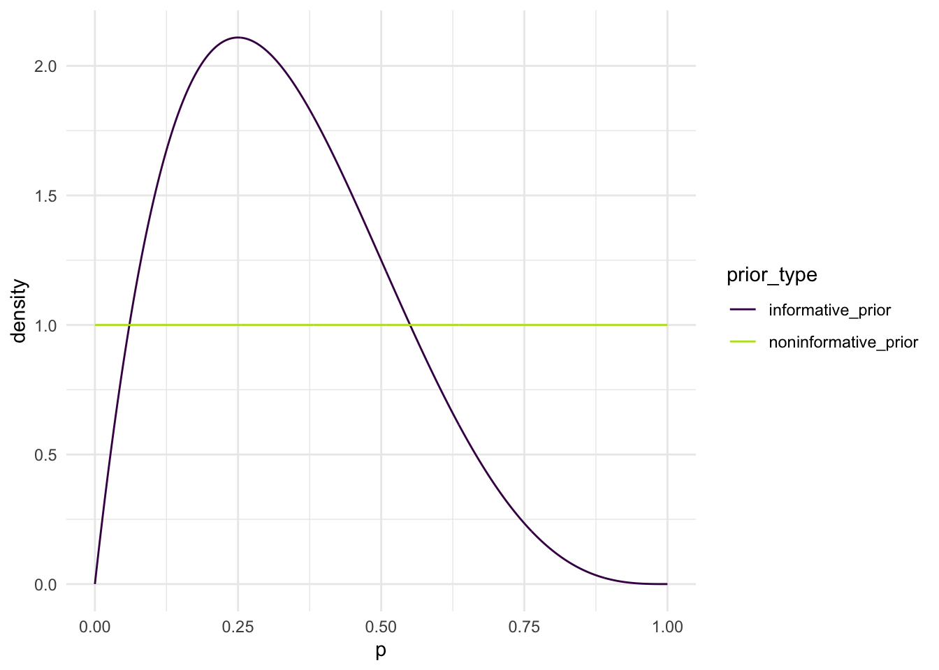
After you have settled on your informative prior, use the code below to construct a plot of both the informative prior and the non-informative prior.
library(tidyverse)ps<-seq(0, 1, length.out =1000)informative_alpha<-2## CHANGE THIS TO YOUR ALPHAinformative_beta<-4## CHANGE THIS TO YOUR BETAnoninformative_alpha<-1noninformative_beta<-1informative_prior<-dbeta(ps, informative_alpha,informative_beta)noninformative_prior<-dbeta(ps,noninformative_alpha, noninformative_beta)prior_plot<-tibble(ps, informative_prior, noninformative_prior)|>pivot_longer(2:3, names_to ="prior_type", values_to ="density")ggplot(data =prior_plot, aes(x =ps, y =density, colour =prior_type))+geom_line()+scale_colour_viridis_d(end =0.9)+theme_minimal()+labs(x ="p")
Exercise. With our informative prior and our non-informative prior, we will now collect some data to include in our Bayesian analysis. After you collect data, derive the posterior distribution of \(p\) using both the non-informative prior and the informative prior. Then, adjust the code below to produce a plot of your two posterior distributions.
library(tidyverse)ps<-seq(0, 1, length.out =1000)informative_alpha<-2## CHANGE THIS TO YOUR ALPHAinformative_beta<-4## CHANGE THIS TO YOUR BETAnoninformative_alpha<-1noninformative_beta<-1informative_prior<-dbeta(ps, informative_alpha,informative_beta)noninformative_prior<-dbeta(ps,noninformative_alpha, noninformative_beta)## CHANGE THESEinformative_alpha_post<-4informative_beta_post<-4informative_post<-dbeta(ps, informative_alpha_post,informative_beta_post)## CHANGE THESEnoninformative_alpha_post<-2noninformative_beta_post<-2noninformative_post<-dbeta(ps, noninformative_alpha_post,noninformative_beta_post)plot_df<-tibble(ps, informative_prior, noninformative_prior,informative_post, noninformative_post)|>pivot_longer(2:5, names_to ="distribution", values_to ="density")|>separate(distribution, into =c("prior_type", "distribution"))ggplot(data =plot_df, aes(x =ps, y =density, colour =prior_type, linetype =distribution))+geom_line()+scale_colour_viridis_d(end =0.9)+theme_minimal()+labs(x ="p")
Exercise. For each posterior, compute the posterior mean (the Bayes estimate).
Exercise. For each posterior, compute a 95% credible interval for \(p\).
Exercise. Interpret one of the 95% credible intervals in context of the problem.
Exercise. Consider the results from the analysis with your informative prior. Is the mean of the informative prior higher or lower than the mean of the posterior distribution? Why do you think that is?
Exercise. The informative prior that you used was very subjective, based on your own knowledge and thoughts of how well you think you can play flip cup. What do you think can be done to limit the subjectivity of this prior?
Exercise. Suppose that, instead of choosing an informative prior via the app, you instead have a target mean for \(p\) of 0.40 and a target standard deviation for \(p\) of 0.05. Your goal is to find parameters of the Beta distribution that satisfy (approximately) these constraints and use those parameters in the prior. Can you modify the code below to figure out good parameters for this prior?
Recall from probability that we discussed using a Poisson model to model the number of goals that the St. Lawrence women’s hockey team scores in a game. In that class, we assumed that we knew the value of \(\lambda\) in that probability model and we computed a few quantities of interest under that assumption.
Usually, however, \(\lambda\) must be estimated (in a frequentist analysis) using data, or, in a Bayesian analysis, we can provide a probability model for \(\lambda\) itself that is either non-informative or informed by expert opinion or prior data.
Suppose that the women’s hockey coach says that he thinks their team scores about 3 goals per game, on average. When pressed for how “sure” they are of that answer and to give a reasonable range for what values that goal scoring rate is, they reply that they are not quite sure. But, they know that they are almost certain that the scoring rate is no less than 2 goals per game, on average.
As discussed in class, the conjugate prior for Poisson data is the Gamma distribution, which can be used to model \(\lambda\).
Exercise. Using the coach’s information, come up with an informative prior for \(\lambda\) with the Gamma distribution. Note that we will have some decisions to make in how to use the coach’s information to come up with an informative prior!
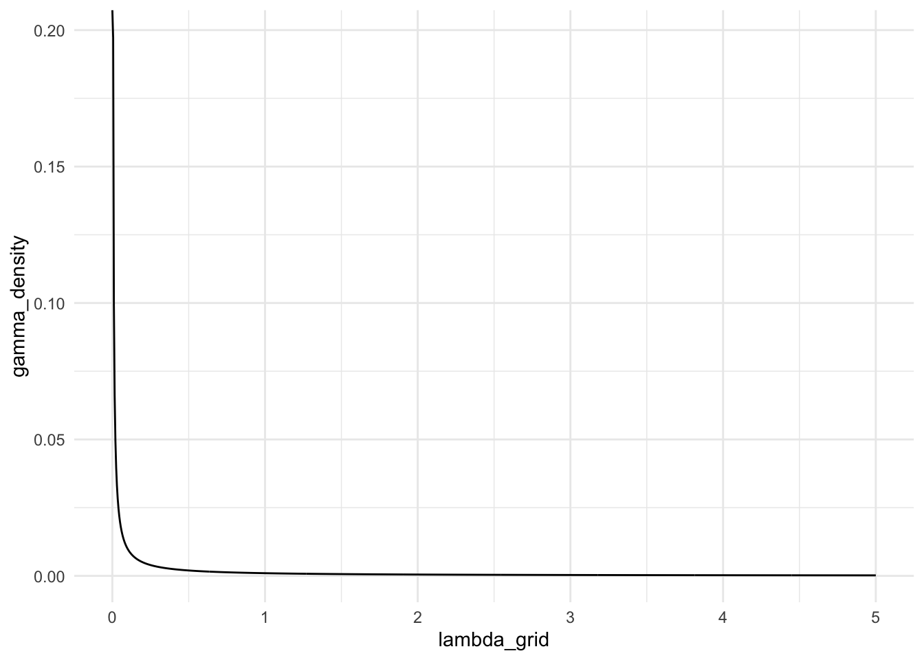
A relatively non-informative prior for \(\lambda\) is a Gamma distribution with very small values for both \(\alpha\) and \(k\). Note that, for the gamma distribution, I am replacing \(\lambda\) with \(k\), so that we are not working with two different \(\lambda\)’s (since the Poisson also has a parameter called \(\lambda\)). Using \(\alpha = 0.001\) and \(k = 0.001\), construct a plot of a relatively non-informative prior for \(\lambda\) using the code below.
Exercise. Based on the plot of the non-informative prior, it’s a little difficult to see why this prior is non-informative. However, using what we derived as the posterior distribution for \(\lambda\), construct an argument for why a prior of \(\alpha = 0.001\) and \(k = 0.001\) is a non-informative prior.
Exercise. Using the code above, construct a plot of the informative prior we derived earlier.
Now suppose that we collect data from the women’s hockey team this season to update both our non-informative prior and our informative prior with data to obtain two posterior distributions for the goal rate.
The code below pulls in data from the season:
library(rvest)url<-"https://saintsathletics.com/sports/womens-ice-hockey/stats/2024-25"tab<-read_html(url)|>html_nodes("table")hockey_stats<-tab[[6]]|>html_table(header =FALSE)newnames<-paste(hockey_stats[1, ], hockey_stats[2, ])goals<-hockey_stats|>set_names(newnames)|>slice(-1, -2)|>mutate(`Shots G` =as.numeric(`Shots G`))|>filter(`Shots G`<=20)|>## filter out the totals (hoping that the women## never scored more than 20 goals in one game!!)pull(`Shots G`)|>as.numeric()goals
Exercise. Using this data and the posterior that we computed in class, figure out the posterior distribution for the goal rate with the non-informative prior and with the informative prior.
Exercise. Use the code below to construct a plot of each of the posterior distributions.
Exercise. What are the mean of the prior distribution, the mean of the data, and the mean of the posterior distribution. Which of these numbers must be in between the other two? Conceptually, why does that make sense?
Exercise. With each posterior, compute a 95% credible interval for \(\lambda\), the rate that the women’s hockey team scores goals.
Exercise. Interpret one of the credible intervals in context of the problem.
Exercise. Think back to the data that we used for this example. What assumptions have we made to complete this analysis? Can you think of ways that we might relax these assumptions?
Mini Project 4: Bayesian Analysis
Project Introduction
AI Usage: You may not use generative AI for this project in any way.
Collaboration: For this project, you may work with a self-contained group of 3. Keep in mind that you may not work with the same person on more than one mini-project (so, if you worked with a student on the first or third mini-project as a partner or in a small group, you may not work with that person on this project). Finally, if working with a partner or in a group of 3, you may submit the same code and the same results/visuals, but your write-ups must be written individually.
Statement of Integrity: At the top of your submission, copy and paste the following statement and type your name, certifying that you have followed all AI and collaboration rules for this mini-project.
“I have followed all rules for collaboration for this project, and I have not used generative AI on this project.”
Rafael Nadal is arguably the greatest men’s clay-court tennis player ever to play the game. In this mini-project, you analyze the probability that Nadal wins a point on his own serve against his primary rival, Novak Djokovic, at the French Open (the most prestigious clay court tournament in the world).
Priors
Before we look at some data, we will consider a few possible prior distributions for the probability that Nadal wins a point on his own serve against Djokovic:
non-informative prior for this probability.
an informative prior based on a clay-court match the two played in the previous year. In that match, Nadal won 46 out of 66 points on his own serve. The standard error of this estimate is 0.05657.
an informative prior based on a sports announcer, who claims that they think Nadal wins about 75% of the points on his serve against Djokovic. They are also “almost sure” that Nadal wins no less than 70% of his points on serve against Djokovic.
Here is some code that we briefly did in class for the Gamma-Poisson hockey scoring example that might help you write code to generate one of the priors mentioned above.
## trying to get a mean of 3 and a probability## that lambda is less than 2 equal to 0.02alphas<-seq(0.01, 100, length.out =2000)ks<-alphas/3target_prob<-0.02prob_less_2<-pgamma(2, alphas, ks)tibble(alphas, ks, prob_less_2)|>mutate(close_to_target =abs(prob_less_2-target_prob))|>filter(close_to_target==min(close_to_target))
Construct a single graph that shows all three of these priors. Note that, for both of the informative priors, there is some subjectivity with how you are going to use the information given to construct an appropriate prior for \(p\), the probability that Nadal wins a point on serve against Djokovic. In other words, for the two informative priors, there is not necessarily a “correct” answer for how to approach creating them. Instead, you will be assessed on your logic and reason in coming up with the two informative priors.
Data
Now, we want to use the 2020 French Open data to update our prior for the probability that Nadal wins a point on serve. In that tournament, the two players played in the final. In that final, Nadal served 84 points and won 56 of those points.
Update each of your three priors with this data and make a plot of the three different posterior distributions of \(p\).
Additionally, for each of the three posteriors, report the posterior mean and 90% credible intervals for \(p\).
Report
For this mini-project, you should submit a report that includes the following:
an introduction to the question of interest that you are answering for this project as well as an overview of how you will be answering this question.
typed work justifying the decisions you made to create the two informative priors. What did you assume when you made those priors?
the graph of the three priors and the graph of the three posteriors, along with any work needed to obtain the posteriors, the posterior means, and the 90% credible intervals
a comparison of the three posteriors.
They should be a bit different from each other: why?
If you had to choose one to use, which one would you choose here and why?
The variance of each posterior should be different. Why do you think one posterior has a lower variance than the other two?
a brief conclusion of what you found in this mini-project.