12 Predictive Modeling with knn
Goals
- explain why it’s necessary to use training data and test data when building a predictive model.
- describe the k-nearest neighbors (knn) procedure.
- interpret a classification table.
- use knn to predict the levels of a categorical response variable for test data.
The structure of this section will be a bit different than the structure of the previous sections. We will complete some of this material on handouts that we will fill in by-hand.
12.1 Introduction to Classification
We will introduce both the knn algorithm and classification in general using a handwritten handout.
12.2 Choosing Predictors and k
We will continue to use the scaled version of the pokemon data set for this handout. This time, we will have 75 pokemon in our training data set and we are only looking at the Steel, Dark, Fire, and Ice types. As discussed in the handout, it is important to scale all of our numeric predictors so that the unit of measurement does not influence the classification results. We can scale all of the numeric variables in a data frame using a combination of across(), where(), and mutate() before we split the data into a training sample and a test sample.
Next, we split the data into a traning sample of 75 pokemon and a test sample.
train_sample <- pokemon |>
  slice_sample(n = 75)

test_sample <- anti_join(pokemon, train_sample)
There are many candidate predictors in this data set: HP, Attack, Defense, …, all the way up to base_experience. How should we determine which predictors to include in our model?
Much of this will be trial and error by evaluating different models with a criterion that we will talk about in the next section. However, it is always helpful to explore the data set with graphics to get us to a good starting point. A scatterplot matrix is a useful exploratory tool. The following is a scatterplot matrix with the response variable, Type, and just three candidate predictors, HP, Attack, and Defense, created with the GGally (“g-g-ally”) package.
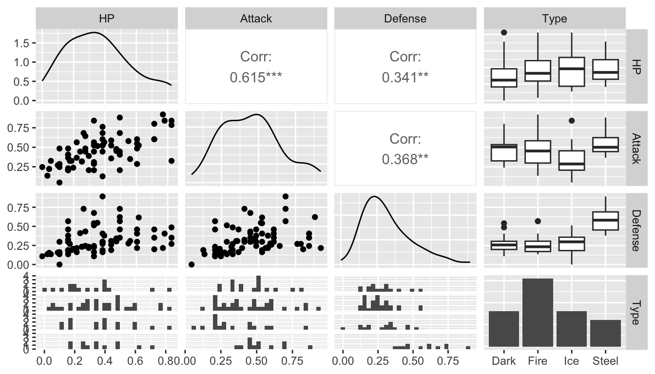
The columns argument is important: it allows you to specify which columns you want to look at. I prefer putting the response, Type (column 3) in the last slot.
We can examine this to see which variables seem to have a relationship with Type. Where would we want to look for this?
What’s given on the diagonal of the scatterplot matrix?
Which variables might we want to include as predictors in a knn model?
Exercise 1. Construct another scatterplot matrix with Type and a different set of predictors. Which predictors look like they might be useful to include in a knn model to predict Type?
After we decide on an initial set of predictors to include, we’ll use the class package to fit a knn model in R. For our first model, let’s just use HP, Attack and Defense as predictors. The kknn library can fit knn models with a kknn() function using syntax similar to lm(), which is used to fit linear models in STAT 213.
The arguments to kknn() are
-
formula, which gives a formula in the styleresponse ~ pred1 + pred2 + .... + predx. For example, if we wantedAttack,DefenseandSpeedto be predictors forType, our formula would beType ~ Attack + Defense + Speed. -
train, a data set with the training data. -
test, a data set with the test data. -
k, the number of nearest neighbors we would like to use in our model.
For those that have taken or are enrolled in STAT 213, this is quite similar to the way you fit regression models with a couple of differences: the function requires 2 data sets instead of 1 (as it requires both a training and a test data set) and the function also requires that we specify a value for \(k\), the number of nearest neighbors to use in our model. The example below fits a knn model with Attack, Defense, and Speed as predictors using \(k = 9\) nearest neighbors.
## fit the knn model with 9 nearest neighbors
knn_mod <- kknn(Type ~ Attack + Defense + Speed, train = train_sample,
                test = test_sample, k = 9)
knn_mod
If you try to run the code above, you will actually get an error! This is one of the rare examples in this class that we see a difference in the way an R function treats <chr> variables and <fct> variables. For the kknn() function to run, the response variable must be a factor and is not allowed to be a character. Let’s make the conversion and then refit the model. Note that, because we have to make the conversion in both the training and the test sample, it will be easier to convert the variable type to factor before we do the split into training and test:
set.seed(1119)

pokemon <- read_csv(here("data", "pokemon_full.csv")) |>
  filter(Type %in% c("Steel", "Dark", "Fire", "Ice")) |>
  mutate(across(where(is.numeric), ~ (.x - min(.x)) /
                                 (max(.x) - min(.x)))) |>
  mutate(Type = as.factor(Type))

train_sample <- pokemon |>
  slice_sample(n = 75)

test_sample <- anti_join(pokemon, train_sample)

knn_mod <- kknn(Type ~ Attack + Defense + Speed, train = train_sample,
                test = test_sample, k = 9)
knn_mod
#>
#> Call:
#> kknn(formula = Type ~ Attack + Defense + Speed, train = train_sample,     test = test_sample, k = 9)
#>
#> Response: "nominal"
The output of knn_mod just gives the formula that we used to fit the data and tells us that the response is “nominal” (which just means that the response is categorical). If we want to examine what the actual classifications are for Pokemon in the test sample, we can pull these out with:
knn_mod$fitted.values
#>  [1] Fire  Fire  Fire  Fire  Ice   Fire  Steel Dark  Fire  Fire  Fire  Fire
#> [13] Steel Dark  Steel Fire  Steel Ice   Steel Fire  Fire  Ice   Fire  Fire
#> [25] Ice   Fire  Dark  Ice   Ice   Steel Fire  Fire  Fire  Fire  Ice   Dark
#> [37] Fire  Fire  Fire  Steel Fire  Ice   Steel Steel Fire
#> Levels: Dark Fire Ice Steel
So, the first pokemon in the test sample is predicted to be Fire type, the second is predicted to be Fire type, etc, the fifth is predicted to be Ice type, etc.
12.3 Evaluating a Predictive Model
But, how well did our model classify pokemon into Types? We still need a metric to evaluate models with different predictors. One definition of a “good” model in the classification context is a model that has a high proportion of correct predictions in the test data set. This should make some intuitive sense, as we would hope that a “good” model correctly classifies most Dark pokemon as Dark, most Fire pokemon as Fire, etc.
In order to examine the performance of a particular model, we’ll create a classification table that shows the results of the model’s classification on observations in the test data set. An equivalent name for the confusion matrix is a confusion matrix.
We can compare the predictions from the knn model with the actual pokemon Types in the test sample with table(), which makes the classification table:
table(knn_mod$fitted.values, test_sample$Type)
#>
#>         Dark Fire Ice Steel
#>   Dark     2    2   0     0
#>   Fire     7   12   3     2
#>   Ice      3    1   1     3
#>   Steel    0    1   3     5
The columns of the classification table give the actual Pokemon types in the test data while the rows give the predicted types from our knn model.
Exercise 2. Interpret the value of 12 in the classification table above.
Exercise 3. Interpret the value of 3 in the column with Dark and the row with Ice.
Exercise 4. Interpret the value of 0 in the bottom-left of the classification table above.
One common metric used to assess overall model performance is the model’s classification rate, which is computed as the number of correct classifications divided by the total number of observations in the test data set.
Exercise 5. Compute the classification rate “by hand” (that is, by using R as a calculator).
Code to automatically obtain the classification rate from a confusion matrix is
What does diag() seem to do in the code above?
Exercise 6. Change the predictors used or change k to improve the classification rate of the model with k = 9 and Attack, Defense, HP, and Speed as predictors.
Exercise 7. A baseline classification rate to compare to is a model that just classifies everything in the test data set as the most common Type in the training data set. In this case, what would the “baseline” classification rate be?
Exercise 8. We will choose \(k\), the number of neighbors considered, using a bit of trial and error, but we will also automate the process by writing a for loop to loop through different values of \(k\). However, we should discuss the relative advantages of smaller and larger k values. Which value is “best” is entirely dependent on the data at hand! What are some advantages for making k smaller? What are some advantages for making k larger?
12.4 Practice
12.4.1 Class Exercises
Examine the following code that fits a knn model using the pokemon data set with \(k\) set to \(9\). For this example, we are using the full pokemon data set (with all Types), so, we might expect our classification rate to be a bit lower.
library(tidyverse)
pokemon <- read_csv(here::here("data/pokemon_full.csv")) |>
mutate(Type = as.factor(Type))
set.seed(1119)
## scale the quantitative predictors
pokemon_scaled <- pokemon |>
mutate(across(where(is.numeric), ~ (.x - min(.x)) /
(max(.x) - min(.x))))
train_sample <- pokemon_scaled |>
slice_sample(n = 550)
test_sample <- anti_join(pokemon_scaled, train_sample)
library(kknn)
knn_mod <- kknn(Type ~ HP + Attack + Defense + Speed + SpAtk + SpDef + height + weight,
train = train_sample, test = test_sample, k = 9)
knn_mod
tab <- table(knn_mod$fitted.values, test_sample$Type)
sum(diag(tab)) / sum(tab)If we want to automate generating a classification rate for a knn model with particular predictors, we have two major choices: write a function and map() across different values of \(k\) or loop through different values of \(k\) with a for loop.
Class Exercise 1. First, we will take a functional programming approach, by writing a function and “mapping” different values of \(k\) through that function. The following code writes a function called get_class_rate that has just a single argument: k_val
Run the code and then test the function by running
get_class_rate(k_val = 10), which should return the classification rate using10nearest neighbors.Together, we will define a vector of k values that we want to map through the function and then write code to perform the mapping using the
map()function from thepurrrpackage.
- Put the classification rates, along with the vector of k values into a
tibble().
- Make a line plot that shows how the classification rate changes for different values of
k.
The code below gives an equivalent way to map or loop through values of \(k\) using a for loop. If you have taken CS 140, you should be able to see a lot of similarities between how loops are defiend in R and how they are defined in Python.
## define an empty vector to store results
class_rate <- double()

## define values of k that we want to loop through
k_vec <- 1:100

for (i in 1:100) {
  knn_mod <- kknn(Type ~ HP + Attack + Defense + Speed + SpAtk + SpDef + height + weight,
                  train = train_sample, test = test_sample, k = k_vec[i])

  knn_mod

  tab <- table(knn_mod$fitted.values, test_sample$Type)

  ## for the ith value of k_vec, store the classification rate as
  ## the ith value of class_rate
  class_rate[i] <- sum(diag(tab)) / sum(tab)
}

class_rate
12.4.2 Your Turn
There will be no your turn exercises for this section. Instead, you will apply some of these concepts in your third project.