12 Dates with `lubridate`

Goals:

use lubridate functions to convert a character variable to a <date> variable.
use lubridate functions to extract useful information from a <date> variable, including the year, month, day of the week, and day of the year.

12.1 Converting Variables to `<date>`

The lubridate package is built to easily work with Date objects and DateTime objects. R does not actually have a class that stores Time objects (unless you install a separate package). Dates tend to be much more common than Times, so, we will primarily focus on Dates, but most functions we will see have easy extensions to Times.

To begin, install the lubridate package, and load the package with library(). The today() function prints today’s date while now() prints today’s date and time. These can sometimes be useful in other contexts, but we will just run the code to see how R stores dates and date-times.

library(tidyverse)
library(lubridate)
today()
#> [1] "2024-08-04"
now()
#> [1] "2024-08-04 06:21:17 EDT"

This first section will deal with how to convert a variable in R to be a Date. We will use a data set that has the holidays of Animal Crossing from January to April. The columns in this data set are:

Holiday, the name of the holiday and
various other columns with different date formats

Read in the data set with

library(here)
holiday_df <- read_csv(here("data/animal_crossing_holidays.csv"))
holiday_df
#> # A tibble: 6 × 10
#>   Holiday         Date1     Date2  Date3 Date4 Date5 Month  Year   Day Month2
#>   <chr>           <chr>     <chr>  <chr> <chr> <chr> <dbl> <dbl> <dbl> <chr> 
#> 1 New Year's Day  1-Jan-20  Jan-1… 1/1/… 1/1/… 2020…     1  2020     1 Janua…
#> 2 Groundhog Day   2-Feb-20  Feb-2… 2/2/… 2/2/… 2020…     2  2020     2 Febru…
#> 3 Valentine's Day 14-Feb-20 Feb-1… 2/14… 2020… 2020…     2  2020    14 Febru…
#> 4 Shamrock Day    17-Mar-20 Mar-1… 3/17… 2020… 2020…     3  2020    17 March 
#> 5 Bunny Day       12-Apr-20 Apr-1… 4/12… 12/4… 2020…     4  2020    12 April 
#> 6 Earth Day       22-Apr-20 Apr-2… 4/22… 2020… 2020…     4  2020    22 April

Which columns were specified as Dates? In this example, none of the columns have the <date> specification: all of the date columns are read in as character variables.

12.1.1 From `<chr>` to `<date>`

We will use the dmy() series of functions in lubridate to convert character variables to dates.

There are a series of dmy()-type variables, each corresponding to a different Day-Month-Year order.

dmy() is used to parse a date from a character vector that has the day first, month second, and year last.
ymd() is used to parse a date that has year first, month second, and date last
ydm() is used to parse a date that has year first, day second, and month last,….

and dym(), mdy(), and myd() work similarly. lubridate is usually “smart” and picks up dates in all kinds of different formats (e.g. it can pick up specifying October as the month and Oct as the month and 10 as the month).

Important

We will typically pair these lubridate functions with a mutate() statement: much like the forcats functions, we are almost always creating a new variable.

Let’s try it out on Date1 and Date2:

holiday_df |> mutate(Date_test = dmy(Date1)) |>
  select(Date_test, everything())
#> # A tibble: 6 × 11
#>   Date_test  Holiday   Date1 Date2 Date3 Date4 Date5 Month  Year   Day Month2
#>   <date>     <chr>     <chr> <chr> <chr> <chr> <chr> <dbl> <dbl> <dbl> <chr> 
#> 1 2020-01-01 New Year… 1-Ja… Jan-… 1/1/… 1/1/… 2020…     1  2020     1 Janua…
#> 2 2020-02-02 Groundho… 2-Fe… Feb-… 2/2/… 2/2/… 2020…     2  2020     2 Febru…
#> 3 2020-02-14 Valentin… 14-F… Feb-… 2/14… 2020… 2020…     2  2020    14 Febru…
#> 4 2020-03-17 Shamrock… 17-M… Mar-… 3/17… 2020… 2020…     3  2020    17 March 
#> 5 2020-04-12 Bunny Day 12-A… Apr-… 4/12… 12/4… 2020…     4  2020    12 April 
#> 6 2020-04-22 Earth Day 22-A… Apr-… 4/22… 2020… 2020…     4  2020    22 April
holiday_df |> mutate(Date_test = mdy(Date2)) |>
  select(Date_test, everything())
#> # A tibble: 6 × 11
#>   Date_test  Holiday   Date1 Date2 Date3 Date4 Date5 Month  Year   Day Month2
#>   <date>     <chr>     <chr> <chr> <chr> <chr> <chr> <dbl> <dbl> <dbl> <chr> 
#> 1 2020-01-01 New Year… 1-Ja… Jan-… 1/1/… 1/1/… 2020…     1  2020     1 Janua…
#> 2 2020-02-02 Groundho… 2-Fe… Feb-… 2/2/… 2/2/… 2020…     2  2020     2 Febru…
#> 3 2020-02-14 Valentin… 14-F… Feb-… 2/14… 2020… 2020…     2  2020    14 Febru…
#> 4 2020-03-17 Shamrock… 17-M… Mar-… 3/17… 2020… 2020…     3  2020    17 March 
#> 5 2020-04-12 Bunny Day 12-A… Apr-… 4/12… 12/4… 2020…     4  2020    12 April 
#> 6 2020-04-22 Earth Day 22-A… Apr-… 4/22… 2020… 2020…     4  2020    22 April

A Reminder: Why do <date> objects even matter? Compare the following two plots: one made where the date is in <chr> form and the other where date is in its appropriate <date> form.

ggplot(data = holiday_df, aes(x = Date1, y = Holiday)) +
  geom_point() + 
  theme_minimal()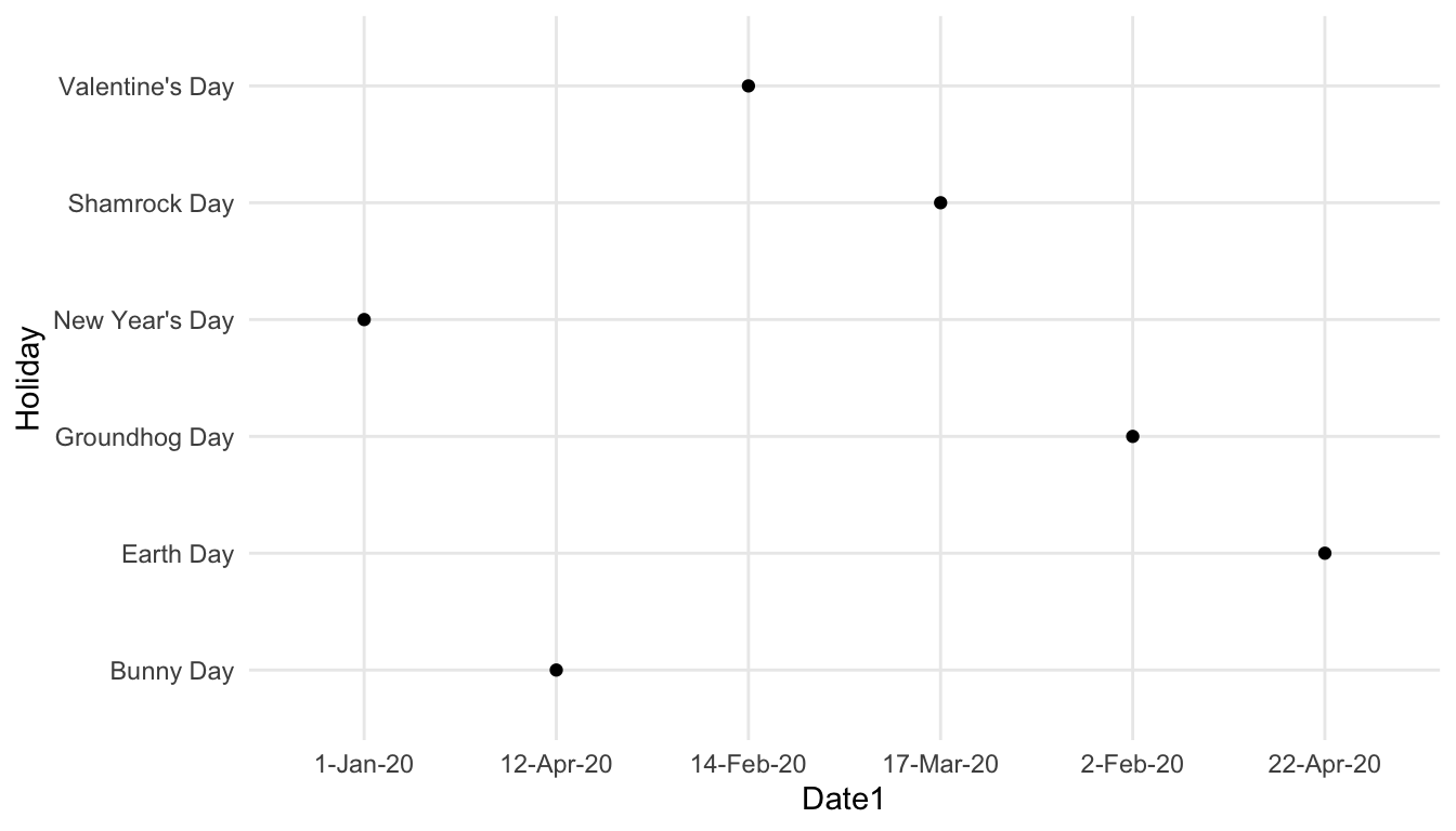


holiday_df <- holiday_df |> mutate(Date_test_plot = dmy(Date1)) |>
  select(Date_test_plot, everything())
ggplot(data = holiday_df, aes(x = Date_test_plot, y = Holiday)) +
  geom_point() +
  theme_minimal()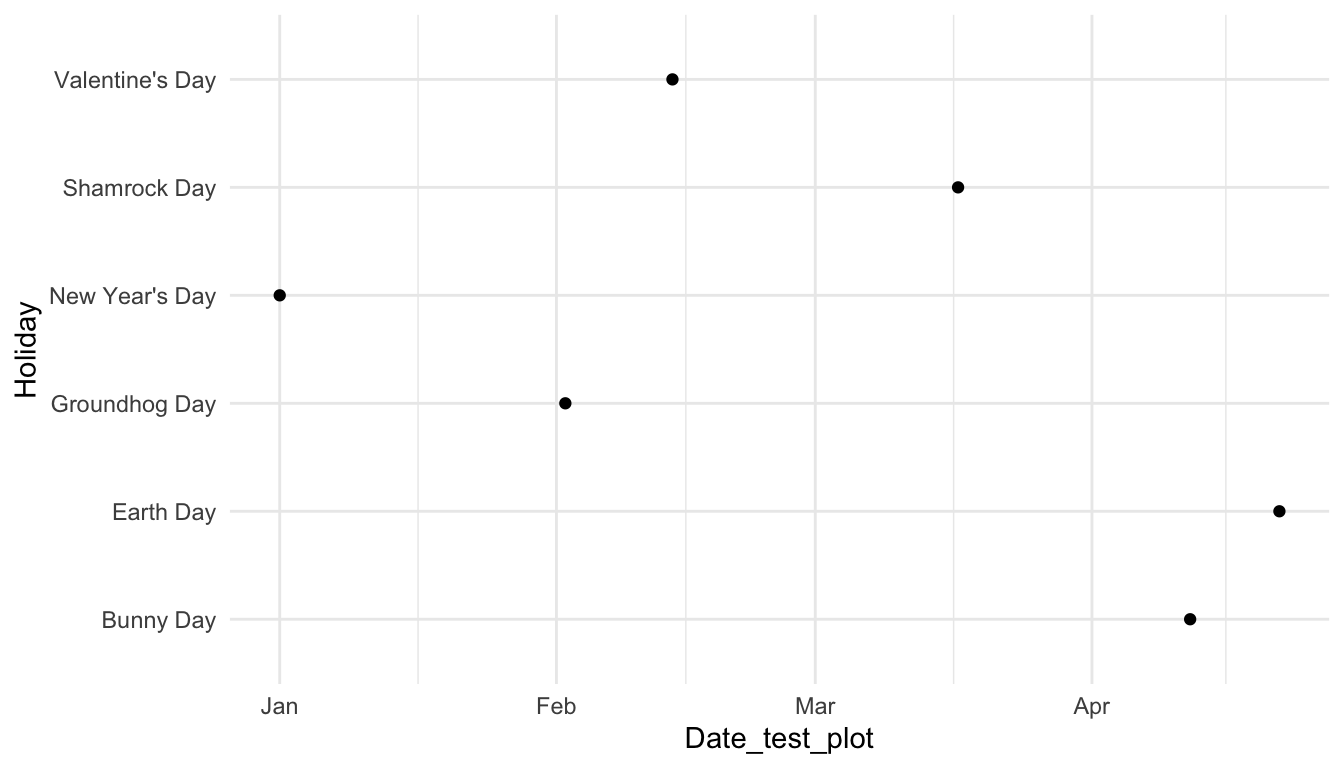

In which plot does the ordering on the x-axis make more sense?

12.1.2 Making a `<date>` variable from Date Components

Another way to create a Date object is to assemble it with make_date() from a month, day, and year components, each stored in a separate column:

holiday_df |> mutate(Date_test2 = make_date(year = Year,
                                             month = Month,
                                             day = Day)) |>
  select(Date_test2, everything())
#> # A tibble: 6 × 12
#>   Date_test2 Date_test_plot Holiday Date1 Date2 Date3 Date4 Date5 Month  Year
#>   <date>     <date>         <chr>   <chr> <chr> <chr> <chr> <chr> <dbl> <dbl>
#> 1 2020-01-01 2020-01-01     New Ye… 1-Ja… Jan-… 1/1/… 1/1/… 2020…     1  2020
#> 2 2020-02-02 2020-02-02     Ground… 2-Fe… Feb-… 2/2/… 2/2/… 2020…     2  2020
#> 3 2020-02-14 2020-02-14     Valent… 14-F… Feb-… 2/14… 2020… 2020…     2  2020
#> 4 2020-03-17 2020-03-17     Shamro… 17-M… Mar-… 3/17… 2020… 2020…     3  2020
#> 5 2020-04-12 2020-04-12     Bunny … 12-A… Apr-… 4/12… 12/4… 2020…     4  2020
#> 6 2020-04-22 2020-04-22     Earth … 22-A… Apr-… 4/22… 2020… 2020…     4  2020
#> # ℹ 2 more variables: Day <dbl>, Month2 <chr>

But, when Month is stored as a character (e.g. February) instead of a number (e.g. 2), problems arise with the make_date() function:

holiday_df |> mutate(Date_test2 = make_date(year = Year,
                                             month = Month2,
                                             day = Day)) |>
  select(Date_test2, everything())
#> # A tibble: 6 × 12
#>   Date_test2 Date_test_plot Holiday Date1 Date2 Date3 Date4 Date5 Month  Year
#>   <date>     <date>         <chr>   <chr> <chr> <chr> <chr> <chr> <dbl> <dbl>
#> 1 NA         2020-01-01     New Ye… 1-Ja… Jan-… 1/1/… 1/1/… 2020…     1  2020
#> 2 NA         2020-02-02     Ground… 2-Fe… Feb-… 2/2/… 2/2/… 2020…     2  2020
#> 3 NA         2020-02-14     Valent… 14-F… Feb-… 2/14… 2020… 2020…     2  2020
#> 4 NA         2020-03-17     Shamro… 17-M… Mar-… 3/17… 2020… 2020…     3  2020
#> 5 NA         2020-04-12     Bunny … 12-A… Apr-… 4/12… 12/4… 2020…     4  2020
#> 6 NA         2020-04-22     Earth … 22-A… Apr-… 4/22… 2020… 2020…     4  2020
#> # ℹ 2 more variables: Day <dbl>, Month2 <chr>

So the make_date() function requires a specific format for the year, month, and day columns. It may take a little pre-processing to put a particular data set in that format.

Exercise 1. What’s the issue with trying to convert Date4 to a <date> form? You may want to investigate Date4 further to answer this question.

holiday_df |> mutate(Date_test = ymd(Date4)) |>
  select(Date_test, everything())
#> # A tibble: 6 × 12
#>   Date_test  Date_test_plot Holiday Date1 Date2 Date3 Date4 Date5 Month  Year
#>   <date>     <date>         <chr>   <chr> <chr> <chr> <chr> <chr> <dbl> <dbl>
#> 1 2001-01-20 2020-01-01     New Ye… 1-Ja… Jan-… 1/1/… 1/1/… 2020…     1  2020
#> 2 2002-02-20 2020-02-02     Ground… 2-Fe… Feb-… 2/2/… 2/2/… 2020…     2  2020
#> 3 NA         2020-02-14     Valent… 14-F… Feb-… 2/14… 2020… 2020…     2  2020
#> 4 NA         2020-03-17     Shamro… 17-M… Mar-… 3/17… 2020… 2020…     3  2020
#> 5 2012-04-20 2020-04-12     Bunny … 12-A… Apr-… 4/12… 12/4… 2020…     4  2020
#> 6 NA         2020-04-22     Earth … 22-A… Apr-… 4/22… 2020… 2020…     4  2020
#> # ℹ 2 more variables: Day <dbl>, Month2 <chr>

Exercise 2. Practice converting Date3 and Date5 to <date> variables with lubridate functions.

12.2 Functions for `<date>` Variables

Once an object is in the <date> format, there are some special functions in lubridate that can be used on that date variable. To investigate some of these functions, we will pull stock market data from Yahoo using the quantmod package. Install the package, and run the following code, which gets stock market price data on Apple, Nintendo, Chipotle, and the S & P 500 Index from 2011 to now.

Note

We have the ability to understand all of the code below, but we will skip over this code for now to focus more on the new information in this section (information about date functions).

## install.packages("quantmod")
library(quantmod)

start <- ymd("2011-01-01")
end <- ymd("2021-5-19")
getSymbols(c("AAPL", "NTDOY", "CMG", "SPY"), src = "yahoo",
           from = start, to = end)
#> [1] "AAPL"  "NTDOY" "CMG"   "SPY"

date_tib <- as_tibble(index(AAPL)) |>
  rename(start_date = value)
app_tib <- as_tibble(AAPL)
nint_tib <- as_tibble(NTDOY)
chip_tib <- as_tibble(CMG)
spy_tib <- as_tibble(SPY)
all_stocks <- bind_cols(date_tib, app_tib, nint_tib, chip_tib, spy_tib)

stocks_long <- all_stocks |>
  select(start_date, AAPL.Adjusted, NTDOY.Adjusted,
                      CMG.Adjusted, SPY.Adjusted) |>
  pivot_longer(2:5, names_to = "Stock_Type", values_to = "Price") |>
  mutate(Stock_Type = fct_recode(Stock_Type,
                                 Apple = "AAPL.Adjusted",
                                 Nintendo = "NTDOY.Adjusted",
                                 Chipotle = "CMG.Adjusted",
                                 `S & P 500` = "SPY.Adjusted"
                                 ))
tail(stocks_long)
#> # A tibble: 6 × 3
#>   start_date Stock_Type Price
#>   <date>     <fct>      <dbl>
#> 1 2021-05-17 Chipotle    26.6
#> 2 2021-05-17 S & P 500  396. 
#> 3 2021-05-18 Apple      123. 
#> 4 2021-05-18 Nintendo    14.1
#> 5 2021-05-18 Chipotle    26.5
#> 6 2021-05-18 S & P 500  393.

You’ll have a chance in class to choose your own stocks to investigate. For now, we’ve made a data set with three variables:

start_date, the opening date for the stock market
Stock_Type, a factor with 4 levels: Apple, Nintendo, Chipotle, and S & P 500
Price, the price of the stock?

First, let’s make a line plot that shows how the S & P 500 has changed over time:

stocks_sp <- stocks_long |> filter(Stock_Type == "S & P 500")
ggplot(data = stocks_sp, aes(x = start_date, y = Price)) +
  geom_line() +
  theme_minimal()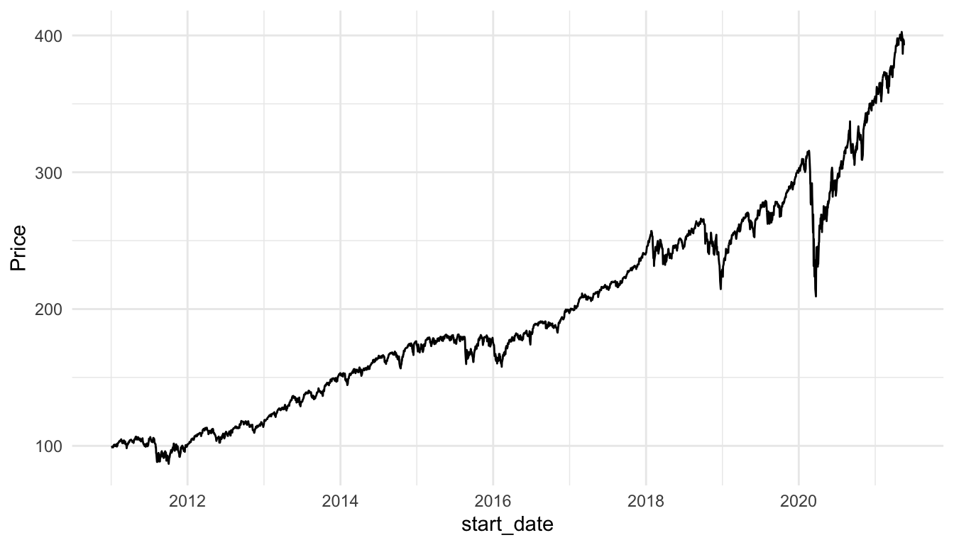

But, there’s other information that we can get from the start_date variable. We might be interested in things like day of the week, monthly trends, or yearly trends. To extract variables like “weekday” and “month” from a <date> variable, there are a series of functions that are fairly straightforward to use. We will discuss the year() month(), mday(), yday(), and wday() functions.

12.2.1 `year()`, `month()`, and `mday()`

The functions year(), month(), and mday() can grab the year, month, and day of the month, respectively, from a <date> variable.

Note

Like the forcats functions and the earlier lubridate functions, the year(), month(), and mday() functions will almost always be paired with a mutate() statement because they will create a new variable.

stocks_long |> mutate(year_stock = year(start_date))
stocks_long |> mutate(month_stock = month(start_date))
stocks_long |> mutate(day_stock = mday(start_date))

12.2.2 `yday()` and `wday()`

The yday() function grabs the day of the year from a <date> object. For example,

test <- mdy("November 4, 2020")
yday(test)
#> [1] 309

returns 309, indicating that November 4th is the 309th day of the year 2020. Using this function in a mutate() statement creates a new variable that has yday for each observation:

stocks_long |> mutate(day_in_year = yday(start_date))
#> # A tibble: 10,444 × 4
#>   start_date Stock_Type Price day_in_year
#>   <date>     <fct>      <dbl>       <dbl>
#> 1 2011-01-03 Apple       9.95           3
#> 2 2011-01-03 Nintendo    7.34           3
#> 3 2011-01-03 Chipotle    4.47           3
#> 4 2011-01-03 S & P 500  99.0            3
#> 5 2011-01-04 Apple      10.0            4
#> 6 2011-01-04 Nintendo    7.10           4
#> # ℹ 10,438 more rows

Finally, the function wday() grabs the day of the week from a <date>. By default, wday() puts the day of the week as a numeric, but I find this confusing, as I can’t ever remember whether a 1 means Sunday or a 1 means Monday. Adding, label = TRUE creates the weekday variable as Sunday, Monday, Tuesday, etc.:

stocks_long |> mutate(day_of_week = wday(start_date))
stocks_long |> mutate(day_of_week = wday(start_date,
                                          label = TRUE, abbr = FALSE))

Possible uses for these functions are:

we want to look at differences between years (with year())
we want to look at differences between months (with month())
we want to look at differences between days of the week (with wday())
we want to see whether there are yearly trends within years (with yday())

Note

Working with times is extremely similar to working with dates. Instead of ymd(), mdy(), etc., you tack on a few extra letters to specify the order that the hour, minute, and seconds appear in the variable: ymd_hms() converts a character vector that has the order year, month, day, hour, minute, second to a <datetime>.

Additionally, the functions hour(), minute(), and second() grab the hour, minute, and second from a <datetime> variable.

Note

Things can get complicated with dates and times, especially if you start to consider things like time duration. Consider how the following might affect an analysis involving time duration:

time zones
leap years (not all years have the same number of days)
differing number of days in a given month
daylight saving time (not all days have the same number of hours)

Exercise 3. The month() function gives the numbers corresponding to each month by default. Type ?month and figure out which argument you would need to change to get the names (January, February, etc.) instead of the month numbers. What about the abbreviations (Jan, Feb, etc.) of each month instead of the month numbers? Try making the changes in the mutate() statement below.

stocks_long |> mutate(month_stock = month(start_date))

12.3 Practice

12.3.1 Class Exercises

Examine the ds_google.csv data, which contains

Month, the year and month from 2004 to now
Data_Science, the relative popularity of data science (Google keeps how it calculates “popularity” as somewhat of a mystery but it is likely based off of the number of times people search for the term “Data Science”)

library(tidyverse)
library(lubridate)
ds_df <- read_csv(here("data/ds_google.csv"))
ds_df
#> # A tibble: 202 × 2
#>   Month   Data_Science
#>   <chr>          <dbl>
#> 1 2004-01           14
#> 2 2004-02            8
#> 3 2004-03           16
#> 4 2004-04           11
#> 5 2004-05            5
#> 6 2004-06            8
#> # ℹ 196 more rows

Class Exercise 1. Use a lubridate function to convert the Month variable to be in the <date> format. Note that, in addition to mdy(), dmy(), ymd(), etc., there are also functions in lubridate like md(), dm(), and ym() that are useful if only two of the three parts of a date are present in a variable.

After converting the Month variable to a date, figure out what R does for the “day” part of the date when it’s not specified in the original variable.

Class Exercise 2. Make a plot of the popularity of Data Science through Time. Add a smoother to your plot. What patterns do you notice?

Class Exercise 3. Modify the code in the tutorial section on the Stocks data to get a data frame on stock prices for the now infamous Gamestop stock. Construct a line plot of the price through time.

Class Exercise 4. Choose one stock and use the lag() function to create a new variable that is the previous day’s stock price for that stock. For what proportion of days was the stock’s closing price higher than it was at close for the day before (indicating that someone who bought shares on Day xxx would have made money at the end of Day xxx + 1).

Class Exercise 5. Those interested in finance/economics might see the naivety of the approach above: usually, the stock market is more thought of as a long-term investment, not a day-to-day investment. For the stock that you selected, adjust your analysis so that you compute the proportion of weeks that a stock’s closing price was higher than it was at close the week before. To simplify things a little, you should only compute this proportion for Wednesdays (and drop the rest of the data).

Class Exercise 6. Those interested in finance/economics might see the naivety of the approach above: usually, the stock market is more thought of as a long-term investment, not a week-to-week investment. For the stock that you selected, adjust your analysis so that you compute the proportion of months that a stock’s closing price was higher than it was at close the month before. To simplify things a little, you should only compute this proportion for the first day of each month (and drop the rest of the data).

12.3.2 Your Turn

The data in the Class Exercises was obtained from Google Trends: Google Trends. Google Trends is incredibly cool to explore, even without R.

Your Turn 1. On Google Trends, Enter in a search term, and change the Time dropdown menu to be 2004-present. Then, enter in a second search term that you want to compare. You can also change the country if you want to (or, you can keep the country as United States).

Note

My search terms will be “super smash” and “animal crossing”, but yours should be something that interests you!

In the top-right window of the graph, you should click the down arrow to download the data set. Delete the first two rows of your data set (either in Excel or R), read in the data set, and change the date variable so that it’s in a Date format.

Your Turn 2. Make a plot of your Popularity variables through time.

Hint (only if you get stuck)

You will need to use a function from tidyr to tidy the data set first.

Your Turn 3. Using your data set that explored a variable or two from 2004 through now, make a table of the average popularity for each year.

Hint (only if you get stuck)

You’ll need a lubridate function to extract the year variable from the date object.

Your Turn 4. Clear your search and now enter a search term that you’d like to investigate for the past 90 days.

Again, click the download button again and read in the data to R. Convert the date variable to be in <date> format.

Your Turn 5. Make a plot of your popularity variable through time, adding a smoother.

12.1 Converting Variables to <date>

12.1.1 From <chr> to <date>

12.1.2 Making a <date> variable from Date Components

12.2 Functions for <date> Variables

12.2.1 year(), month(), and mday()

12.2.2 yday() and wday()

12.3 Practice

12.3.1 Class Exercises

12.3.2 Your Turn

12.1 Converting Variables to `<date>`

12.1.1 From `<chr>` to `<date>`

12.1.2 Making a `<date>` variable from Date Components

12.2 Functions for `<date>` Variables

12.2.1 `year()`, `month()`, and `mday()`

12.2.2 `yday()` and `wday()`