4 Wrangling with `dplyr`

Goals:

Use the mutate(), if_else(), and case_when() functions to create new variables.
Use the filter() and slice(), select(), and arrange() functions in dplyr to choose certain rows to keep or get rid of, choose certain columns to keep or get rid of, and to sort the data, respectively.
Use group_by() and summarise() to create useful summaries of a data set.
Combine the above goals with plotting to explore the babynames data set and a data set on SLU majors.
Explain what the pipe operator |> does and explain when you can and cannot use the pipe operator.

Throughout this chapter, we will use the babynames data set in the babynames R package. To begin, install the babynames package by typing install.packages("babynames") in your bottom-left console winow, and read about the data set by running

library(babynames)

and then typing ?babynames in your bottom-left window of R Studio. We see that this data set contains baby name data provided by the SSA in the United States dating back to 1880:

head(babynames)
#> # A tibble: 6 × 5
#>    year sex   name          n   prop
#>   <dbl> <chr> <chr>     <int>  <dbl>
#> 1  1880 F     Mary       7065 0.0724
#> 2  1880 F     Anna       2604 0.0267
#> 3  1880 F     Emma       2003 0.0205
#> 4  1880 F     Elizabeth  1939 0.0199
#> 5  1880 F     Minnie     1746 0.0179
#> 6  1880 F     Margaret   1578 0.0162

The second data set that we will use has 27 observations, one for each of SLU’s majors and contains 3 variables:

Major, the name of the major.
nfemales, the number of female graduates in that major from 2015 - 2019.
nmales, the number of male graduates in that major from 2015 - 2019.

The data has kindly been provided by Dr. Ramler. With your Notes R Project open, you can read in the data set with

library(tidyverse)
slumajors_df <- read_csv("data/SLU_Majors_15_19.csv")
slumajors_df
#> # A tibble: 27 × 3
#>    Major                        nfemales nmales
#>    <chr>                           <dbl>  <dbl>
#>  1 Anthropology                       34     15
#>  2 Art & Art History                  65     11
#>  3 Biochemistry                       14     11
#>  4 Biology                           162     67
#>  5 Business in the Liberal Arts      135    251
#>  6 Chemistry                          26     14
#>  7 Computer Science                   21     47
#>  8 Conservation Biology               38     20
#>  9 Economics                         128    349
#> 10 English                           131     54
#> # … with 17 more rows

There are many interesting and informative plots that we could make with either data set, but most require some data wrangling first. This chapter will provide the foundation for such wrangling skills.

4.1 `mutate()`: Create Variables

Sometimes, we will want to create a new variable that’s not in the data set, oftentimes using if_else(), case_when(), or basic algebraic operations on one or more of the columns already present in the data set.

R understands the following symbols:

+ for addition, - for subtraction
* for multiplication, / for division
^ for raising something to a power (3 ^ 2 is equal to 9)

R also does the same order of operations as usual: parentheses, then exponents, then multiplication and division, then addition and subtraction.

For example, suppose that we want to create a variable in slumajors_df that has the total number of students graduating in each major. We can do this with mutate():

slumajors_df |> mutate(ntotal = nfemales + nmales)
#> # A tibble: 27 × 4
#>    Major                        nfemales nmales ntotal
#>    <chr>                           <dbl>  <dbl>  <dbl>
#>  1 Anthropology                       34     15     49
#>  2 Art & Art History                  65     11     76
#>  3 Biochemistry                       14     11     25
#>  4 Biology                           162     67    229
#>  5 Business in the Liberal Arts      135    251    386
#>  6 Chemistry                          26     14     40
#>  7 Computer Science                   21     47     68
#>  8 Conservation Biology               38     20     58
#>  9 Economics                         128    349    477
#> 10 English                           131     54    185
#> # … with 17 more rows

There’s a lot to break down in that code chunk: most importantly, we’re seeing our first of many, many, many, many, many, many, many instances of using |> to pipe! The |> operator approximately reads take slumajors_df “and then” mutate() it.

Piping is a really convenient, easy-to-read way to build a sequence of commands. How you can read the above code is:

Take slumajors_df and with slumajors_df,
perform a mutate() step to create the new variable called ntotal, which is nfemales plus nmales.

Since this is our first time using mutate(), let’s also delve into what the function is doing. In general, mutate() reads:

mutate(name_of_new_variable = operations_on_old_variables).

R just automatically assumes that you want to do the operation for every single row in the data set, which is often quite convenient!

We might also want to create a variable that is the percentage of students identifying as female for each major:

slumajors_df |>
  mutate(percfemale = 100 * nfemales / (nfemales + nmales))
#> # A tibble: 27 × 4
#>    Major                        nfemales nmales percfemale
#>    <chr>                           <dbl>  <dbl>      <dbl>
#>  1 Anthropology                       34     15       69.4
#>  2 Art & Art History                  65     11       85.5
#>  3 Biochemistry                       14     11       56  
#>  4 Biology                           162     67       70.7
#>  5 Business in the Liberal Arts      135    251       35.0
#>  6 Chemistry                          26     14       65  
#>  7 Computer Science                   21     47       30.9
#>  8 Conservation Biology               38     20       65.5
#>  9 Economics                         128    349       26.8
#> 10 English                           131     54       70.8
#> # … with 17 more rows

But what happened to ntotal? Is it still in the printout? It’s not: when we created the variable ntotal, we didn’t actually save the new data set as anything. So R makes and prints the new variable, but it doesn’t get saved to any data set. If we want to save the new data set, then we can use the <- operator. Here, we’re saving the new data set with the same name as the old data set: slumajors_df. Then, we’re doing the same thing for the percfemale variable. We won’t always want to give the new data set the same name as the old one: we’ll talk about this more in the chapter exercises.

slumajors_df <- slumajors_df |>
  mutate(percfemale = 100 * nfemales / (nfemales + nmales))

slumajors_df <- slumajors_df |> mutate(ntotal = nfemales + nmales)

But, you can pipe as many things together as you want to, so it’s probably easier to just create both variables in one go. The following chunk says to “Take slumajors_df and create a new variable ntotal. With that new data set, create a new variable called percfemale.” Finally, the slumajors_df <- at the beginning says to “save this new data set as a data set with the same name, slumajors_df.”

slumajors_df <- slumajors_df |>
  mutate(ntotal = nfemales + nmales) |>
  mutate(percfemale = 100 * nfemales / (nfemales + nmales))

4.1.1 `if_else()` and `case_when()`

Suppose that you want to make a new variable that is conditional on another variable (or more than one variable) in the data set. Then we would typically use mutate() coupled with

if_else() if your new variable is created on only one condition
case_when() if your new variable is created on more than one condition

Suppose we want to create a new variable that tells us whether or not the Major has a majority of Women. That is, we want this new variable, morewomen to be "Yes" if the Major has more than 50% women and "No" if it has 50% or less.

slumajors_df |> mutate(morewomen = if_else(percfemale > 50,
                                            true = "Yes",
                                            false = "No"))
#> # A tibble: 27 × 6
#>    Major               nfema…¹ nmales percf…² ntotal morew…³
#>    <chr>                 <dbl>  <dbl>   <dbl>  <dbl> <chr>  
#>  1 Anthropology             34     15    69.4     49 Yes    
#>  2 Art & Art History        65     11    85.5     76 Yes    
#>  3 Biochemistry             14     11    56       25 Yes    
#>  4 Biology                 162     67    70.7    229 Yes    
#>  5 Business in the Li…     135    251    35.0    386 No     
#>  6 Chemistry                26     14    65       40 Yes    
#>  7 Computer Science         21     47    30.9     68 No     
#>  8 Conservation Biolo…      38     20    65.5     58 Yes    
#>  9 Economics               128    349    26.8    477 No     
#> 10 English                 131     54    70.8    185 Yes    
#> # … with 17 more rows, and abbreviated variable names
#> #   ¹nfemales, ²percfemale, ³morewomen

The mutate() statement reads: create a new variable called morewomen that is equal to "Yes" if percfemale > 50 is true and is equal to "No" if perfemale is not > 0.5. The first argument is the condition, the second is what to name the new variable when the condition holds, and the third is what to name the variable if the condition does not hold.

We use conditions all of the time in every day life. For example, New York had a quarantine order stating that people coming from 22 states in July 2020 would need to quarantine. In terms of a condition, this would read “if you are traveling to New York from one of the 22 states, then you need to quarantine for 2 weeks. Else, if not, then you don’t need to quarantine.” The trick in using these conditions in R is getting used to the syntax of the code.

We can see from the above set up that if we had more than one condition, then we’d need to use a different function (or use nested if_else() statements, which can be a nightmare to read). If we have more than one condition for creating the new variable, we will use case_when().

For example, when looking at the output, we see that Biochemistry has 56% female graduates. That’s “about” a 50/50 split, so suppose we want a variable called large_majority that is “female” when the percent women is 70 or more, “male” when the percent women is 30 or less, and “none” when the percent female is between 30 and 70.

slumajors_df |> mutate(large_majority =
                          case_when(percfemale >= 70 ~ "female",
                                    percfemale <= 30 ~ "male",
                                    percfemale > 30 & percfemale < 70 ~ "none")) 
#> # A tibble: 27 × 6
#>    Major               nfema…¹ nmales percf…² ntotal large…³
#>    <chr>                 <dbl>  <dbl>   <dbl>  <dbl> <chr>  
#>  1 Anthropology             34     15    69.4     49 none   
#>  2 Art & Art History        65     11    85.5     76 female 
#>  3 Biochemistry             14     11    56       25 none   
#>  4 Biology                 162     67    70.7    229 female 
#>  5 Business in the Li…     135    251    35.0    386 none   
#>  6 Chemistry                26     14    65       40 none   
#>  7 Computer Science         21     47    30.9     68 none   
#>  8 Conservation Biolo…      38     20    65.5     58 none   
#>  9 Economics               128    349    26.8    477 male   
#> 10 English                 131     54    70.8    185 female 
#> # … with 17 more rows, and abbreviated variable names
#> #   ¹nfemales, ²percfemale, ³large_majority

The case_when() function reads “When the percent female is more than or equal to 70, assign the new variable large_majority the value of”female”, when it’s less or equal to 30, assign the more than 30 and less than 70, assign the variable the value of “none” .” The & is a boolean operator: we’ll talk more about that later so don’t worry too much about that for now.

Let’s save these two new variables to the slumajors_df:

slumajors_df <- slumajors_df |>
  mutate(morewomen = if_else(percfemale > 50,
                             true = "Yes",
                             false = "No")) |>
  mutate(large_majority =
           case_when(percfemale >= 70 ~ "female",
                     percfemale <= 30 ~ "male",
                     percfemale > 30 & percfemale < 70 ~ "none"))

4.1.2 Exercises

Exercises marked with an * indicate that the exercise has a solution at the end of the chapter at 4.7.

Do you think it is ethical to exclude non-binary genders from analyses and graphs in the slumajors data set? Why or why not?
* Create a new variable that is called major_size and is “large” when the total number of majors is 100 or more and “small” when the total number of majors is less than 100.
Create a new variable that is called major_size2 and is “large when the total number of majors is 150 or more,”medium” when the total number of majors is between 41 and 149, and “small” when the total number of majors is 40 or fewer.
About 55% of SLU students identify as female. So, in the definition of the morewomen variable, does it make more sense to use 55% as the cutoff or 50%?
* Investigate what happens with case_when() when you give overlapping conditions and when you give conditions that don’t cover all observations. For overlapping conditions, create a variable testcase that is "Yes" when percfemale is greater than or equal to 40 and "No" when percfemale is greater than 60 For conditions that don’t cover all observations, create a variable testcase2 that is "Yes" when percfemale is greater than or equal to 55 and "No" when percfemale is less than 35.
With one or two of the newly created variables from mutate(), create a plot that investigates a question of interest you might have about the data.

4.2 `arrange()` (Ordering Rows), `select()` (Choosing Columns), and `slice()` and `filter()` (Choosing Rows)

arrange() is used to order rows in the data set according to some variable, select() is used to choose columns to keep (or get rid of) and filter() is used to keep (or get rid of) only some of the observations (rows).

4.2.1 `arrange()`: Ordering Rows

The arrange() function allows us to order rows in the data set using one or more variables. The function is very straightforward. Suppose that we want to order the rows so that the majors with the lowest percfemale are first:

slumajors_df |> arrange(percfemale)
#> # A tibble: 27 × 7
#>    Major       nfema…¹ nmales percf…² ntotal morew…³ large…⁴
#>    <chr>         <dbl>  <dbl>   <dbl>  <dbl> <chr>   <chr>  
#>  1 Economics       128    349    26.8    477 No      male   
#>  2 Physics           6     14    30       20 No      male   
#>  3 Computer S…      21     47    30.9     68 No      none   
#>  4 Business i…     135    251    35.0    386 No      none   
#>  5 Music            13     21    38.2     34 No      none   
#>  6 Geology          28     41    40.6     69 No      none   
#>  7 History          62     82    43.1    144 No      none   
#>  8 Philosophy       24     29    45.3     53 No      none   
#>  9 Mathematics      74     83    47.1    157 No      none   
#> 10 Government      127    116    52.3    243 Yes     none   
#> # … with 17 more rows, and abbreviated variable names
#> #   ¹nfemales, ²percfemale, ³morewomen, ⁴large_majority

Which major has the lowest percentage of female graduates?

We see that, by default, arrange() orders the rows from low to high. To order from high to low so that the majors with the highest percfemale are first, use desc() around the variable that you are ordering by:

slumajors_df |> arrange(desc(percfemale))
#> # A tibble: 27 × 7
#>    Major       nfema…¹ nmales percf…² ntotal morew…³ large…⁴
#>    <chr>         <dbl>  <dbl>   <dbl>  <dbl> <chr>   <chr>  
#>  1 Art & Art …      65     11    85.5     76 Yes     female 
#>  2 Psychology      278     61    82.0    339 Yes     female 
#>  3 French           27      7    79.4     34 Yes     female 
#>  4 Spanish          35     10    77.8     45 Yes     female 
#>  5 Statistics       28      9    75.7     37 Yes     female 
#>  6 Global Stu…      69     27    71.9     96 Yes     female 
#>  7 Neuroscien…      61     24    71.8     85 Yes     female 
#>  8 Performanc…     144     57    71.6    201 Yes     female 
#>  9 Religious …      10      4    71.4     14 Yes     female 
#> 10 English         131     54    70.8    185 Yes     female 
#> # … with 17 more rows, and abbreviated variable names
#> #   ¹nfemales, ²percfemale, ³morewomen, ⁴large_majority

What is the major with the highest percentage of women graduates?

4.2.2 `select()` Choose Columns

We might also be interested in getting rid of some of the columns in a data set. One reason to do this is if there are an overwhelming (30+) columns in a data set, but we know that we just need a few of them. The easiest way to use select() is to just input the names of the columns that you want to keep. For example, if we were only interested in majors and their totals, we could do

slumajors_df |> select(Major, ntotal)
#> # A tibble: 27 × 2
#>    Major                        ntotal
#>    <chr>                         <dbl>
#>  1 Anthropology                     49
#>  2 Art & Art History                76
#>  3 Biochemistry                     25
#>  4 Biology                         229
#>  5 Business in the Liberal Arts    386
#>  6 Chemistry                        40
#>  7 Computer Science                 68
#>  8 Conservation Biology             58
#>  9 Economics                       477
#> 10 English                         185
#> # … with 17 more rows

If I wanted to use this data set for anything else, I’d also need to name, or rename, it with <-. We would probably want to name it something other than slumajors_df so as to not overwrite the original data set, in case we want to use those other variables again later!

We might also want to use select() to get rid of one or two columns. If this is the case, we denote any column you want to get rid of with -. For example, we might want to get rid of the ntotal column that we made and get rid of the nmales and nfemales columns:

slumajors_df |> select(-ntotal, -nfemales, -nmales)
#> # A tibble: 27 × 4
#>    Major                        percfemale morewomen large…¹
#>    <chr>                             <dbl> <chr>     <chr>  
#>  1 Anthropology                       69.4 Yes       none   
#>  2 Art & Art History                  85.5 Yes       female 
#>  3 Biochemistry                       56   Yes       none   
#>  4 Biology                            70.7 Yes       female 
#>  5 Business in the Liberal Arts       35.0 No        none   
#>  6 Chemistry                          65   Yes       none   
#>  7 Computer Science                   30.9 No        none   
#>  8 Conservation Biology               65.5 Yes       none   
#>  9 Economics                          26.8 No        male   
#> 10 English                            70.8 Yes       female 
#> # … with 17 more rows, and abbreviated variable name
#> #   ¹large_majority

select() comes with many useful helper functions, but these are oftentimes not needed. One of the helper functions that is actually often useful is everything(). We can, for example, use this after using mutate() to put the variable that was just created at the front of the data set to make sure there weren’t any unexpected issues:

slumajors_df |> mutate(propfemale = percfemale / 100) |>
  select(propfemale, everything())
#> # A tibble: 27 × 8
#>    propfemale Major    nfema…¹ nmales percf…² ntotal morew…³
#>         <dbl> <chr>      <dbl>  <dbl>   <dbl>  <dbl> <chr>  
#>  1      0.694 Anthrop…      34     15    69.4     49 Yes    
#>  2      0.855 Art & A…      65     11    85.5     76 Yes    
#>  3      0.56  Biochem…      14     11    56       25 Yes    
#>  4      0.707 Biology      162     67    70.7    229 Yes    
#>  5      0.350 Busines…     135    251    35.0    386 No     
#>  6      0.65  Chemist…      26     14    65       40 Yes    
#>  7      0.309 Compute…      21     47    30.9     68 No     
#>  8      0.655 Conserv…      38     20    65.5     58 Yes    
#>  9      0.268 Economi…     128    349    26.8    477 No     
#> 10      0.708 English      131     54    70.8    185 Yes    
#> # … with 17 more rows, 1 more variable:
#> #   large_majority <chr>, and abbreviated variable names
#> #   ¹nfemales, ²percfemale, ³morewomen

Verify that propfemale now appears first in the data set. everything() tacks on all of the remaining variables after propfemale. So, in this case, it’s a useful way to re-order the columns so that what you might be most interested in appears first.

4.2.3 `slice()` and `filter()`: Choose Rows

Instead of choosing which columns to keep, we can also choose certain rows to keep using either slice() or filter().

slice() allows you to specify the row numbers corresponding to rows that you want to keep. For example, suppose that we only want to keep the rows with the five most popular majors:

slumajors_df |> arrange(desc(ntotal)) |>
  slice(1, 2, 3, 4, 5)
#> # A tibble: 5 × 7
#>   Major        nfema…¹ nmales percf…² ntotal morew…³ large…⁴
#>   <chr>          <dbl>  <dbl>   <dbl>  <dbl> <chr>   <chr>  
#> 1 Economics        128    349    26.8    477 No      male   
#> 2 Business in…     135    251    35.0    386 No      none   
#> 3 Psychology       278     61    82.0    339 Yes     female 
#> 4 Government       127    116    52.3    243 Yes     none   
#> 5 Biology          162     67    70.7    229 Yes     female 
#> # … with abbreviated variable names ¹nfemales, ²percfemale,
#> #   ³morewomen, ⁴large_majority

We can alternatively use slice(1:5), which is shorthand for slice(1, 2, 3, 4, 5). While slice() is useful, it is relatively simple. We’ll come back to it again in a few weeks as well when we discuss subsetting in base R.

filter() is a way to keep rows by specifying a condition related to one or more of the variables in the data set. We’ve already seen conditions in if_else() and case_when() statements, but they’ll now be used to “filter” the rows in our data set.

We can keep rows based on a categorical variable or a quantitative variable or a combination of any number of categorical and quantitative variables. R uses the following symbols to make comparisons. We’ve already been using the more intuitive symbols (like < and >):

< and <= for less than and less than or equal to, respectively
> and >= for greater than and greater than or equal to, respectively
== for equal to (careful: equal to is a double equal sign ==)
!= for not equal to (in general, ! denotes “not”)

It’s probably time for a change of data set too! We’ll be working with the babynames data set for the rest of this chapter:

library(babynames)
babynames
#> # A tibble: 1,924,665 × 5
#>     year sex   name          n   prop
#>    <dbl> <chr> <chr>     <int>  <dbl>
#>  1  1880 F     Mary       7065 0.0724
#>  2  1880 F     Anna       2604 0.0267
#>  3  1880 F     Emma       2003 0.0205
#>  4  1880 F     Elizabeth  1939 0.0199
#>  5  1880 F     Minnie     1746 0.0179
#>  6  1880 F     Margaret   1578 0.0162
#>  7  1880 F     Ida        1472 0.0151
#>  8  1880 F     Alice      1414 0.0145
#>  9  1880 F     Bertha     1320 0.0135
#> 10  1880 F     Sarah      1288 0.0132
#> # … with 1,924,655 more rows

If needed, we can remind ourselves what is in the babynames data set by typing ?babynames in the console window.

What do the following statements do? See if you can guess before running the code.

babynames |> filter(name == "Matthew")
babynames |> filter(year >= 2000)
babynames |> filter(sex != "M")
babynames |> filter(prop > 0.05)
babynames |> filter(year == max(year))

Why are some things put in quotes, like "Matthew" while some things aren’t, like 2000? Can you make out a pattern?

We can also combine conditions on multiple variables in filter() using Boolean operators. We’ve already seen one of these in the case_when() statement above: & means “and”.

Look at the Venn diagrams in R for Data Science to learn about the various Boolean operators you can use in R: https://r4ds.had.co.nz/transform.html#logical-operators. The Boolean operators can be used in other functions in R as well, as we’ve already seen with if_else() and case_when().

The following gives some examples. See if you can figure out what each line of code is doing before running it.

babynames |> filter(n > 20000 | prop > 0.05)
babynames |> filter(sex == "F" & name == "Mary")
babynames |> filter(sex == "F" & name == "Mary" & prop > 0.05)

4.2.4 Exercises

Exercises marked with an * indicate that the exercise has a solution at the end of the chapter at 4.7.

What happens when you arrange() by one of the categorical variables in the slumajors_df data set?
* Use select() and everything() to put the large_majority variable as the first column in the slumajors_df data set.
* In the babynames data set, use filter(), mutate() with rank(), and arrange() to print the 10 most popular Male babynames in 2017.
In the babynames data set, use filter() to keep only the rows with your name (or, another name that interests you) and one sex (either "M" or "F"). Name the new data set something and then construct a line plot that looks at the either the n or prop of your chosen name through year.

4.3 `summarise()` and `group_by()`: Create Summaries

The summarise() function is useful to get summaries from the data. For example, suppose that we want to know the average major size at SLU across the five year span or the total number of majors across those five years. Then we can use summarise() and a summary function, like mean(), sum(), median(), max(), min(), n(), etc. You’ll notice that the format of summarise() is extremely similar to the format of mutate(). Using the slumajors_df data again just for one quick example,

slumajors_df |>
  summarise(meantotalmajor = mean(ntotal),
            totalgrad = sum(ntotal))
#> # A tibble: 1 × 2
#>   meantotalmajor totalgrad
#>            <dbl>     <dbl>
#> 1           124.      3347

4.3.1 `group_by()`: Groups

summarise() is often most useful when paired with a group_by() statement. Doing so allows us to get summaries across different groups.

For example, suppose that you wanted the total number of registered births per year in the babynames data set:

babynames |> group_by(year) |>
  summarise(totalbirths = sum(n))
#> # A tibble: 138 × 2
#>     year totalbirths
#>    <dbl>       <int>
#>  1  1880      201484
#>  2  1881      192696
#>  3  1882      221533
#>  4  1883      216946
#>  5  1884      243462
#>  6  1885      240854
#>  7  1886      255317
#>  8  1887      247394
#>  9  1888      299473
#> 10  1889      288946
#> # … with 128 more rows

group_by() takes a grouping variable, and then, using summarise() computes the given summary function on each group.

Most summary functions are intuitive if you’ve had intro stat. But, if you’re not sure whether the summary for getting the maximum is maximum() or max(), just try both!

The n() function can be used within summarise() to obtain the number of observations. It will give you the total number of rows, if used without group_by()

babynames |> summarise(totalobs = n())
#> # A tibble: 1 × 1
#>   totalobs
#>      <int>
#> 1  1924665

Note that n() typically doesn’t have any inputs. It’s typically more useful when paired with group_by(): this allows us to see the number of observations within each year, for instance:

babynames |> group_by(year) |>
  summarise(ngroup = n())
#> # A tibble: 138 × 2
#>     year ngroup
#>    <dbl>  <int>
#>  1  1880   2000
#>  2  1881   1935
#>  3  1882   2127
#>  4  1883   2084
#>  5  1884   2297
#>  6  1885   2294
#>  7  1886   2392
#>  8  1887   2373
#>  9  1888   2651
#> 10  1889   2590
#> # … with 128 more rows

4.3.2 Exercises

Exercises marked with an * indicate that the exercise has a solution at the end of the chapter at 4.7.

Compare summarise() with mutate() using the following code. What’s the difference between the two functions?

slumajors_df |>
  summarise(meantotalmajor = mean(ntotal),
            totalgrad = sum(ntotal)) 
slumajors_df |>
  mutate(meantotalmajor = mean(ntotal),
            totalgrad = sum(ntotal)) |>
  select(meantotalmajor, totalgrad, everything())

Using the data set from the group_by() and n() combination,

babynames |> group_by(year) |>
  summarise(ngroup = n())
#> # A tibble: 138 × 2
#>     year ngroup
#>    <dbl>  <int>
#>  1  1880   2000
#>  2  1881   1935
#>  3  1882   2127
#>  4  1883   2084
#>  5  1884   2297
#>  6  1885   2294
#>  7  1886   2392
#>  8  1887   2373
#>  9  1888   2651
#> 10  1889   2590
#> # … with 128 more rows

make a line plot with ngroup on the x-axis and year on the y-axis. How would you interpret the plot?

* Create a data set that has a column for name and a column that shows the total number of births for that name across all years and both sexes.
* group_by() can also be used with other functions, including mutate(). Use group_by() and mutate() to rank the names from most to least popular in each year-sex combination.
* From the data set in 4, filter() the data to keep only the most popular name in each year-sex combination and then construct a summary table showing how many times each name appears as the most popular name.
* Run the following code. Intuitively, a slice(1, 2, 3, 4, 5) should grab the first five rows of the data set, but, when we try to run that, we get 1380 rows. Try to figure out what the issue is by using Google to search something like “dplyr not slicing correctly after using group by.” What do you find?

babynames_test <- babynames |>
  group_by(year, sex) |> mutate(ntest = n / prop)
babynames_test |> slice(1, 2, 3, 4, 5)
#> # A tibble: 1,380 × 6
#> # Groups:   year, sex [276]
#>     year sex   name          n   prop   ntest
#>    <dbl> <chr> <chr>     <int>  <dbl>   <dbl>
#>  1  1880 F     Mary       7065 0.0724  97605.
#>  2  1880 F     Anna       2604 0.0267  97605.
#>  3  1880 F     Emma       2003 0.0205  97605.
#>  4  1880 F     Elizabeth  1939 0.0199  97605.
#>  5  1880 F     Minnie     1746 0.0179  97605.
#>  6  1880 M     John       9655 0.0815 118400.
#>  7  1880 M     William    9532 0.0805 118400.
#>  8  1880 M     James      5927 0.0501 118400.
#>  9  1880 M     Charles    5348 0.0452 118400.
#> 10  1880 M     George     5126 0.0433 118400.
#> # … with 1,370 more rows

4.4 Missing Values

Both of the data sets that we’ve worked with are nice in that they do not have any missing values. We’ll see plenty of examples of data sets with missing values later, so we should examine how the various functions that we’ve talked about so far tackle missing values.

Missing values in R are denoted with NA for “Not Available.” Run the following code to create a toy data set with some missing values so that we can see how the various functions we’ve used so far deal with NA values.

toy_df <- tibble(x = c(NA, 3, 4, 7),
                 y = c(1, 4, 3, 2),
                 z = c("A", "A", "B", NA))
toy_df
#> # A tibble: 4 × 3
#>       x     y z    
#>   <dbl> <dbl> <chr>
#> 1    NA     1 A    
#> 2     3     4 A    
#> 3     4     3 B    
#> 4     7     2 <NA>

4.4.1 Exercises

Exercises marked with an * indicate that the exercise has a solution at the end of the chapter at 4.7.

* mutate(). Try to create a new variable with mutate() involving x. What does R do with the missing value?
arrange(). Try arranging the data set by x. What does R do with the missing value?
filter(). Try filtering so that only observations where x is less than 5 are kept. What does R do with the missing value?
summarise(). Try using summarise() with a function involving x. What does R return?
group_by() and summarise(). To your statement in 4, add a group_by(z) statement before your summarise(). What does R return now?

4.4.2 Removing Missing Values

Missing values should not be removed without carefully examination and a note of what the consequences might be (e.g. why are these values missing?). We have a toy data set that is meaningless, so we aren’t asking those questions now, but we will for any data set that does have missing values!

If we have investigated the missing values and are comfortable with removing them, many functions that we would use in summarise() have an na.rm argument that we can set to TRUE to tell summarise() to remove any NAs before taking the mean(), median(), max(), etc.

toy_df |> summarise(meanx = mean(x, na.rm = TRUE))
#> # A tibble: 1 × 1
#>   meanx
#>   <dbl>
#> 1  4.67

If we want to remove the missing values more directly, we can use the is.na() function in combination with filter(). If the variable is NA (Not Available) for an observation, is.na() evaluates to TRUE; if not, is.na() evaluates to FALSE. Test this out using mutate() to create a new variable for whether Median is missing:

toy_df |> mutate(missingx = is.na(x))
#> # A tibble: 4 × 4
#>       x     y z     missingx
#>   <dbl> <dbl> <chr> <lgl>   
#> 1    NA     1 A     TRUE    
#> 2     3     4 A     FALSE   
#> 3     4     3 B     FALSE   
#> 4     7     2 <NA>  FALSE

missingx is TRUE only for the the first observation. We can use this to our advantage with filter() to filter it out of the data set, without going through the extra step of actually making a new variable missingx:

toy_df |> filter(is.na(x) != TRUE)
#> # A tibble: 3 × 3
#>       x     y z    
#>   <dbl> <dbl> <chr>
#> 1     3     4 A    
#> 2     4     3 B    
#> 3     7     2 <NA>

You’ll commonly see this written as short-hand in people’s code you may come across as:

toy_df |> filter(!is.na(x))
#> # A tibble: 3 × 3
#>       x     y z    
#>   <dbl> <dbl> <chr>
#> 1     3     4 A    
#> 2     4     3 B    
#> 3     7     2 <NA>

which says to “keep anything that does not have a missing x value” (recall that the ! means “not”).

4.5 More about the Pipe

We are jumping straight into using piping, but we do want to have an appreciation on how terrible life would be without it. What piping does is make whatever is given before the |> pipe the first argument of whatever function follows the |>. So

df |> mutate(x = y + 4)

is equivalent to

mutate(df, x = y + 4)

It might also help to use an analogy when thinking about piping. Consider the Ke$ha’s morning routine in the opening of the song Tik Tok. If we were to write her morning routine in terms of piping,

kesha |> wake_up(time = "morning", feels_like = "P-Diddy") |>
  grab(glasses) |>
  brush(teeth, item = "jack", unit = "bottle") |> ....

Kesha first wakes up in the morning, and then the Kesha that has woken up grabs her glasses, and then the Kesha who has woken up and has her glasses brushes her teeth, etc.

The pipe operator |> is loaded automatically with R. We’ve been using the pipe quite a bit, but let’s delve a little deeper into what it’s actually doing. We will use the videogame_clean.csv data file, which contains variables on video games from 2004 - 2019, including

game, the name of the game
release_date, the release date of the game
release_date2, a second coding of release date
price, the price in dollars,
owners, the number of owners (given in a range)
median_playtime, the median playtime of the game
metascore, the score from the website Metacritic
price_cat, 1 for Low (less than 10.00 dollars), 2 for Moderate (between 10 and 29.99 dollars), and 3 for High (30.00 or more dollars)
meta_cat, Metacritic’s review system, with the following categories: “Overwhelming Dislike”, “Generally Unfavorable”, “Mixed Reviews”, “Generally Favorable”, “Universal Acclaim”.
playtime_miss, whether median play time is missing (TRUE) or not (FALSE)

Load in the data set with

videogame_df <- read_csv("data/videogame_clean.csv")
#> Rows: 26688 Columns: 15
#> ── Column specification ────────────────────────────────────
#> Delimiter: ","
#> chr  (7): game, release_date, owners, meta_cat, develope...
#> dbl  (6): price, median_playtime, metascore, price_cat, ...
#> lgl  (1): playtime_miss
#> date (1): release_date2
#> 
#> ℹ Use `spec()` to retrieve the full column specification for this data.
#> ℹ Specify the column types or set `show_col_types = FALSE` to quiet this message.
head(videogame_df)
#> # A tibble: 6 × 15
#>   game       relea…¹ release_…² price owners media…³ metas…⁴
#>   <chr>      <chr>   <date>     <dbl> <chr>    <dbl>   <dbl>
#> 1 Half-Life… Nov 16… 2004-11-16  9.99 10,00…      66      96
#> 2 Counter-S… Nov 1,… 2004-11-01  9.99 10,00…     128      88
#> 3 Counter-S… Mar 1,… 2004-03-01  9.99 10,00…       3      65
#> 4 Half-Life… Nov 1,… 2004-11-01  4.99 5,000…       0      NA
#> 5 Half-Life… Jun 1,… 2004-06-01  9.99 2,000…       0      NA
#> 6 CS2D       Dec 24… 2004-12-24 NA    1,000…      10      NA
#> # … with 8 more variables: price_cat <dbl>, meta_cat <chr>,
#> #   playtime_miss <lgl>, number <dbl>, developer <chr>,
#> #   publisher <chr>, average_playtime <dbl>,
#> #   meta_cat_factor <chr>, and abbreviated variable names
#> #   ¹release_date, ²release_date2, ³median_playtime,
#> #   ⁴metascore

Let’s say we want to filter() the data set to include only videogames with a metascore that isn’t missing. We’ve been using code like

videogame_df |> filter(!is.na(metascore))

What the pipe is doing is putting videogame_df as the first argument in the filter() function so that the piping statement in the chunk above is equivalent to:

filter(videogame_df, !is.na(metascore))

If we want to first filter out games with a non-missing metascore, get rid of all observations with a median play time of 0, and then obtain the “median” median_playtime for each of the 3 price categories, we would typically use

videogame_df |> filter(!is.na(metascore)) |>
  filter(median_playtime > 0) |>
  group_by(price_cat) |>
  summarise(avg_med_time = median(median_playtime, na.rm = TRUE))

We see from the summary that, in general, games do tend to give you more “bang for the buck”: more expensive games tend to have a larger median play time. Consecutive pipes build on each other: we can slowly build out what the pipe is doing step-by-step. Starting from the top, videogame_df is the first argument in the filter(!is.na(metascore)) function:

filter(videogame_df, !is.na(metascore))

filter(videogame_df, !is.na(metascore)) is the first argument in filter(median_playtime > 0):

filter(filter(videogame_df, !is.na(metascore)), median_playtime > 0)

filter(filter(videogame_df, !is.na(metascore)), median_playtime > 0) is the first argument in group_by(price_cat):

group_by(filter(filter(videogame_df, !is.na(metascore)),
                median_playtime > 0), price_cat)

and group_by(filter(filter(videogame_df, !is.na(metascore)), median_playtime > 0), price_cat) is the first argument of summarise(avg_med_time = median(median_playtime, na.rm = TRUE)):

summarise(group_by(filter(filter(videogame_df, !is.na(metascore)),
  median_playtime > 0), price_cat), 
  avg_med_time = median(median_playtime, na.rm = TRUE))

and we obtain the same result without the |> pipe. So, why use the pipe? Compare the code the uses the pipe operator to find the average median playtime to the code that doesn’t. Which is easier to read? Which do you think is easier to write? The example shows that, for our purposes, the pipe is most useful in aiding the readability of our code. It’s a lot easier to see what’s happening in the code chunk with the pipes than it is in the previous code chunk without the pipe because, with the pipe, we can read the code from left to right and top to bottom. Without the pipe, we need to read the code from the “inside to the outside”, which is much more challenging.

4.5.1 When You Can’t Use the Pipe

So, the pipe is a convenient way to put what precedes the pipe as the first argument to the function that follows the pipe. It’s important to understand this as you learn more about R because, while the functions in tidyverse are purposefully made to make good use of the pipe, not all functions in R utilize the pipe. Most of the functions in the tidyverse have a first argument that is a data set (which is why we can use pipes consecutively), but this isn’t the case with all R functions.

For example, if you have taken STAT 213, you’ve used lm() to fit many different types of linear models. If you haven’t taken STAT 213, lm(response ~ explanatory, data = name_of_data_set) stands for “linear model” and can be used to fit the simple linear regression model that you learned about in STAT 113. You might expect something like this to work:

videogame_df |> lm(metascore ~ price)
#> Error in as.data.frame.default(data): cannot coerce class '"formula"' to a data.frame

But it throws us an error. Typing in ?lm reveals that its first argument is a formula to fit the model, not a data set. So the function is trying to run

lm(videogame_df, metascore ~ price)
#> Error in as.data.frame.default(data): cannot coerce class '"formula"' to a data.frame

which doesn’t work because the arguments to the function are mixed up (the formula should appear first and the data set should appear second).

For one final note about the pipe, note that the pipe operator |> is relatively new. Previously, the primary pipe operator used was %>% and came from the magrittr package. For almost all cases, the two operators are equivalent. However, when scanning the Internet for help with code, you will probably see |> used in many of people’s responses on sites like StackOverflow.

4.5.2 Exercises

Exercises marked with an * indicate that the exercise has a solution at the end of the chapter at 4.7.

* Recode the following to look cleaner by using the pipe |>.

fitness_df <- read_csv("data/higham_fitness_clean.csv")
#> Rows: 993 Columns: 9
#> ── Column specification ────────────────────────────────────
#> Delimiter: ","
#> chr  (2): month, weekday
#> dbl  (6): active_cals, distance, flights, steps, dayofye...
#> date (1): Start
#> 
#> ℹ Use `spec()` to retrieve the full column specification for this data.
#> ℹ Specify the column types or set `show_col_types = FALSE` to quiet this message.
summarise(group_by(filter(fitness_df, weekday == "Sat" | weekday == "Sun"),
                   month),
          meanweekend = mean(distance, na.rm = TRUE)) 
#> # A tibble: 12 × 2
#>    month meanweekend
#>    <chr>       <dbl>
#>  1 Apr          5.30
#>  2 Aug          5.52
#>  3 Dec          3.30
#>  4 Feb          4.87
#>  5 Jan          3.89
#>  6 Jul          4.85
#>  7 Jun          4.18
#>  8 Mar          4.86
#>  9 May          5.00
#> 10 Nov          3.06
#> 11 Oct          3.82
#> 12 Sep          4.02

Explain why the following code gives a warning message and returns NA. Use the list of Arguments in ?mean in your explanation.

fitness_df |> mean(distance, na.rm = TRUE)
#> [1] NA

4.6 Chapter Exercises

We found both in the SLU majors data set and in the FiveThirtyEight majors data set that Statistics has a higher proportion of women than almost all other STEM fields. Read the first two sections of this article. Write 2-3 sentences about the article’s reasoning of why there are more women in statistics than in other STEM fields.
* a. Choose 5 names that interest you and create a new data set that only has data on those 5 names.

Use group_by() and summarise() to add together the number of Females and Males for each name in each year. Hint: you can group_by() more than one variable!
Make a line plot showing the popularity of these 5 names over time.

1. Choose a year and a sex that interests you and filter the data set to only contain observations from that year and sex.

Create a new variable that ranks the names from most popular to least popular.
Create a bar plot that shows the 10 most popular names as well as the count for each name.

* In some cases throughout this chapter, we’ve renamed data sets using <- with the same name like

toy_df <- toy_df |> mutate(newvar = x / y)

In other cases, we’ve given the data set a new name, like

toy_small <- toy_df |> filter(!is.na(x))

For which of the functions below is a generally “safe” to name the data set using the same name after using the function. Why?

Pose a question about the babynames data set and then answer your question with either a graphic or a data summary.

4.7 Exercise Solutions

4.7.1 `mutate()` S

* Create a new variable that is called major_size and is “large” when the total number of majors is 100 or more and “small” when the total number of majors is less than 100.

slumajors_df |> mutate(major_size = if_else(ntotal >= 100,
                                             true = "large",
                                             false = "small"))
#> # A tibble: 27 × 8
#>    Major       nfema…¹ nmales percf…² ntotal morew…³ large…⁴
#>    <chr>         <dbl>  <dbl>   <dbl>  <dbl> <chr>   <chr>  
#>  1 Anthropolo…      34     15    69.4     49 Yes     none   
#>  2 Art & Art …      65     11    85.5     76 Yes     female 
#>  3 Biochemist…      14     11    56       25 Yes     none   
#>  4 Biology         162     67    70.7    229 Yes     female 
#>  5 Business i…     135    251    35.0    386 No      none   
#>  6 Chemistry        26     14    65       40 Yes     none   
#>  7 Computer S…      21     47    30.9     68 No      none   
#>  8 Conservati…      38     20    65.5     58 Yes     none   
#>  9 Economics       128    349    26.8    477 No      male   
#> 10 English         131     54    70.8    185 Yes     female 
#> # … with 17 more rows, 1 more variable: major_size <chr>,
#> #   and abbreviated variable names ¹nfemales, ²percfemale,
#> #   ³morewomen, ⁴large_majority
## OR
slumajors_df |>
  mutate(major_size = case_when(ntotal >= 100 ~ "large",
                                ntotal < 100 ~ "small"))
#> # A tibble: 27 × 8
#>    Major       nfema…¹ nmales percf…² ntotal morew…³ large…⁴
#>    <chr>         <dbl>  <dbl>   <dbl>  <dbl> <chr>   <chr>  
#>  1 Anthropolo…      34     15    69.4     49 Yes     none   
#>  2 Art & Art …      65     11    85.5     76 Yes     female 
#>  3 Biochemist…      14     11    56       25 Yes     none   
#>  4 Biology         162     67    70.7    229 Yes     female 
#>  5 Business i…     135    251    35.0    386 No      none   
#>  6 Chemistry        26     14    65       40 Yes     none   
#>  7 Computer S…      21     47    30.9     68 No      none   
#>  8 Conservati…      38     20    65.5     58 Yes     none   
#>  9 Economics       128    349    26.8    477 No      male   
#> 10 English         131     54    70.8    185 Yes     female 
#> # … with 17 more rows, 1 more variable: major_size <chr>,
#> #   and abbreviated variable names ¹nfemales, ²percfemale,
#> #   ³morewomen, ⁴large_majority

* Investigate what happens with case_when() when you give overlapping conditions and when you give conditions that don’t cover all observations. For overlapping conditions, create a variable testcase that is "Yes" when percfemale is greater than or equal to 40 and "No" when percfemale is greater than 60 For conditions that don’t cover all observations, create a variable testcase2 that is "Yes" when percefemale is greater than or equal to 55 and "No" when percfemale is less than 35.

#> # A tibble: 27 × 9
#>    Major       nfema…¹ nmales percf…² ntotal morew…³ large…⁴
#>    <chr>         <dbl>  <dbl>   <dbl>  <dbl> <chr>   <chr>  
#>  1 Anthropolo…      34     15    69.4     49 Yes     none   
#>  2 Art & Art …      65     11    85.5     76 Yes     female 
#>  3 Biochemist…      14     11    56       25 Yes     none   
#>  4 Biology         162     67    70.7    229 Yes     female 
#>  5 Business i…     135    251    35.0    386 No      none   
#>  6 Chemistry        26     14    65       40 Yes     none   
#>  7 Computer S…      21     47    30.9     68 No      none   
#>  8 Conservati…      38     20    65.5     58 Yes     none   
#>  9 Economics       128    349    26.8    477 No      male   
#> 10 English         131     54    70.8    185 Yes     female 
#> # … with 17 more rows, 2 more variables: testcase <chr>,
#> #   testcase2 <chr>, and abbreviated variable names
#> #   ¹nfemales, ²percfemale, ³morewomen, ⁴large_majority

For overlapping cases, case_when prioritizes the first case given.

For non-coverage, any observation that is not covered is given an NA.

4.7.2 `arrange()`, `select()`, …. S

* Use select() and everything() to put the large_majority variable as the first column in the slumajors_df data set.

slumajors_df |> select(large_majority, everything())
#> # A tibble: 27 × 7
#>    large_major…¹ Major nfema…² nmales percf…³ ntotal morew…⁴
#>    <chr>         <chr>   <dbl>  <dbl>   <dbl>  <dbl> <chr>  
#>  1 none          Anth…      34     15    69.4     49 Yes    
#>  2 female        Art …      65     11    85.5     76 Yes    
#>  3 none          Bioc…      14     11    56       25 Yes    
#>  4 female        Biol…     162     67    70.7    229 Yes    
#>  5 none          Busi…     135    251    35.0    386 No     
#>  6 none          Chem…      26     14    65       40 Yes    
#>  7 none          Comp…      21     47    30.9     68 No     
#>  8 none          Cons…      38     20    65.5     58 Yes    
#>  9 male          Econ…     128    349    26.8    477 No     
#> 10 female        Engl…     131     54    70.8    185 Yes    
#> # … with 17 more rows, and abbreviated variable names
#> #   ¹large_majority, ²nfemales, ³percfemale, ⁴morewomen

* In the babynames data set, use filter(), mutate() with rank(), and arrange() to print the 10 most popular Male babynames in 2017.

babynames |> filter(sex == "M" & year == 2017) |>
  mutate(rankname = rank(desc(n))) |>
  filter(rankname <= 10)
#> # A tibble: 10 × 6
#>     year sex   name         n    prop rankname
#>    <dbl> <chr> <chr>    <int>   <dbl>    <dbl>
#>  1  2017 M     Liam     18728 0.00954        1
#>  2  2017 M     Noah     18326 0.00933        2
#>  3  2017 M     William  14904 0.00759        3
#>  4  2017 M     James    14232 0.00725        4
#>  5  2017 M     Logan    13974 0.00712        5
#>  6  2017 M     Benjamin 13733 0.00699        6
#>  7  2017 M     Mason    13502 0.00688        7
#>  8  2017 M     Elijah   13268 0.00676        8
#>  9  2017 M     Oliver   13141 0.00669        9
#> 10  2017 M     Jacob    13106 0.00668       10

4.7.3 `summarise()` and `group_by()` S

* Create a data set that has a column for name and a column that shows the total number of births for that name across all years and both sexes.

babynames |> group_by(name) |>
  summarise(totalbirths = sum(n))
#> # A tibble: 97,310 × 2
#>    name      totalbirths
#>    <chr>           <int>
#>  1 Aaban             107
#>  2 Aabha              35
#>  3 Aabid              10
#>  4 Aabir               5
#>  5 Aabriella          32
#>  6 Aada                5
#>  7 Aadam             254
#>  8 Aadan             130
#>  9 Aadarsh           199
#> 10 Aaden            4658
#> # … with 97,300 more rows

* group_by() can also be used with other functions, including mutate(). Use group_by() and mutate() to rank the names from most to least popular in each year-sex combination.

ranked_babynames <- babynames |> group_by(year, sex) |>
  mutate(rankname = rank((desc(n))))

* From the data set in 4, filter() the data to keep only the most popular name in each year-sex combination and then construct a summary table showing how many times each name appears as the most popular name.

ranked_babynames |> filter(rankname == 1) |>
  group_by(name) |>
  summarise(nappear = n()) |>
  arrange(desc(nappear))
#> # A tibble: 18 × 2
#>    name     nappear
#>    <chr>      <int>
#>  1 Mary          76
#>  2 John          44
#>  3 Michael       44
#>  4 Robert        17
#>  5 Jennifer      15
#>  6 Jacob         14
#>  7 James         13
#>  8 Emily         12
#>  9 Jessica        9
#> 10 Lisa           8
#> 11 Linda          6
#> 12 Emma           5
#> 13 Noah           4
#> 14 Sophia         3
#> 15 Ashley         2
#> 16 Isabella       2
#> 17 David          1
#> 18 Liam           1

* Run the following code. Intuitively, a slice(1, 2, 3, 4, 5) should grab the first five rows of the data set, but, when we try to run that, we get 1380 rows. Try to figure out what the issue is by using Google to search something like “dplyr not slicing correctly after using group by.” What do you find?

babynames_test <- babynames |>
  group_by(year, sex) |> mutate(ntest = n / prop)
babynames_test |> slice(1, 2, 3, 4, 5)
#> # A tibble: 1,380 × 6
#> # Groups:   year, sex [276]
#>     year sex   name          n   prop   ntest
#>    <dbl> <chr> <chr>     <int>  <dbl>   <dbl>
#>  1  1880 F     Mary       7065 0.0724  97605.
#>  2  1880 F     Anna       2604 0.0267  97605.
#>  3  1880 F     Emma       2003 0.0205  97605.
#>  4  1880 F     Elizabeth  1939 0.0199  97605.
#>  5  1880 F     Minnie     1746 0.0179  97605.
#>  6  1880 M     John       9655 0.0815 118400.
#>  7  1880 M     William    9532 0.0805 118400.
#>  8  1880 M     James      5927 0.0501 118400.
#>  9  1880 M     Charles    5348 0.0452 118400.
#> 10  1880 M     George     5126 0.0433 118400.
#> # … with 1,370 more rows

Functions like slice() and rank() operate on defined groups in the data set if using a function like group_by() first. Sometimes this feature is quite convenient. But, if we no longer want slice() or rank() or other functions to account for these groups, we need to add an ungroup() pipe, which simply drops the groups that we had formed:

babynames_test |> ungroup() |> slice(1:5)
#> # A tibble: 5 × 6
#>    year sex   name          n   prop  ntest
#>   <dbl> <chr> <chr>     <int>  <dbl>  <dbl>
#> 1  1880 F     Mary       7065 0.0724 97605.
#> 2  1880 F     Anna       2604 0.0267 97605.
#> 3  1880 F     Emma       2003 0.0205 97605.
#> 4  1880 F     Elizabeth  1939 0.0199 97605.
#> 5  1880 F     Minnie     1746 0.0179 97605.

4.7.4 Missing Values S

* mutate(). Try to create a new variable with mutate() involving x. What does R do with the missing value?

toy_df |> mutate(xy = x * y)
#> # A tibble: 4 × 5
#>       x     y z     newvar    xy
#>   <dbl> <dbl> <chr>  <dbl> <dbl>
#> 1    NA     1 A      NA       NA
#> 2     3     4 A       0.75    12
#> 3     4     3 B       1.33    12
#> 4     7     2 <NA>    3.5     14

R puts another NA in place of x times y for the observation with the missing x.

4.7.5 Piping S

* Recode the following to look cleaner by using the pipe |>:

fitness_df <- read_csv("data/higham_fitness_clean.csv")
#> Rows: 993 Columns: 9
#> ── Column specification ────────────────────────────────────
#> Delimiter: ","
#> chr  (2): month, weekday
#> dbl  (6): active_cals, distance, flights, steps, dayofye...
#> date (1): Start
#> 
#> ℹ Use `spec()` to retrieve the full column specification for this data.
#> ℹ Specify the column types or set `show_col_types = FALSE` to quiet this message.
summarise(group_by(filter(fitness_df, weekday == 1 | weekday == 7),
                   month),
          meanweekend = mean(distance, na.rm = TRUE)) 
#> # A tibble: 0 × 2
#> # … with 2 variables: month <chr>, meanweekend <dbl>

fitness_df |> filter(weekday == 1 | weekday == 7) |>
  group_by(month) |>
  summarise(meanweekend = mean(distance, na.rm = TRUE)) 
#> # A tibble: 0 × 2
#> # … with 2 variables: month <chr>, meanweekend <dbl>

4.7.6 Chapter Exercises S

* a. Choose 5 names that interest you and create a new data set that only has data on those 5 names.

Use group_by() and summarise() to add together the number of Females and Males for each name in each year. Hint: you can group_by() more than one variable!
Make a line plot showing the popularity of these 5 names over time.

baby5 <- babynames |> filter(name == "Matthew" | name == "Ivan" |
                                name == "Jessica" | name == "Robin" |
                                name == "Michael")
baby5_tot <- baby5 |> group_by(year, name) |>
  summarise(ntot = sum(n))
#> `summarise()` has grouped output by 'year'. You can
#> override using the `.groups` argument.
ggplot(data = baby5_tot, aes(x = year, y = ntot, colour = name)) +
  geom_line()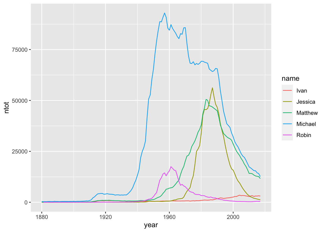

* In some cases throughout this chapter, we’ve renamed data sets using <- with the same name like

toy_df <- toy_df |> mutate(newvar = x / y)

In other cases, we’ve given the data set a new name, like

toy_small <- toy_df |> filter(!is.na(x))

For which of the functions below is a generally “safe” to name the data set using the same name after using the function. Why?

mutate()

Usually fine: mutating creates a new variable, which doesn’t change any of the other variables in the data set, if things get messed up with the new variable.

arrange()

Usually fine: ordering the rows a certain way won’t change any plots and doesn’t change any of the underlying data.

filter()

Usually not the best practice. Naming the data set the same name after the filter means that you permanently lose data that you filtered out, unless you re-read in the data set at the beginning.

summarise()

Usually not the best practice. Again, naming the summarized data set the same as the original data means that you lose the original data, unless you re-read it in at the beginning. For example,

toy_df <- toy_df |> summarise(meanx = mean(x))
toy_df
#> # A tibble: 1 × 1
#>   meanx
#>   <dbl>
#> 1    NA

means that we now have no way to access the original data in toy_df.

select()

This can sometimes be okay if you’re sure that the variables you are removing won’t ever be used.

4.8 Non-Exercise `R` Code

library(babynames)
head(babynames)
library(tidyverse)
slumajors_df <- read_csv("data/SLU_Majors_15_19.csv")
slumajors_df
slumajors_df |> mutate(ntotal = nfemales + nmales)
slumajors_df |>
  mutate(percfemale = 100 * nfemales / (nfemales + nmales))
slumajors_df <- slumajors_df |>
  mutate(percfemale = 100 * nfemales / (nfemales + nmales))
slumajors_df <- slumajors_df |> mutate(ntotal = nfemales + nmales)
slumajors_df <- slumajors_df |>
  mutate(ntotal = nfemales + nmales) |>
  mutate(percfemale = 100 * nfemales / (nfemales + nmales))
slumajors_df |> mutate(morewomen = if_else(percfemale > 50,
                                            true = "Yes",
                                            false = "No"))
slumajors_df |> mutate(large_majority =
                          case_when(percfemale >= 70 ~ "female",
                                    percfemale <= 30 ~ "male",
                                    percfemale > 30 & percfemale < 70 ~ "none")) 
slumajors_df <- slumajors_df |>
  mutate(morewomen = if_else(percfemale > 50,
                             true = "Yes",
                             false = "No")) |>
  mutate(large_majority =
           case_when(percfemale >= 70 ~ "female",
                     percfemale <= 30 ~ "male",
                     percfemale > 30 & percfemale < 70 ~ "none")) 
slumajors_df |> arrange(percfemale)
slumajors_df |> arrange(desc(percfemale))
slumajors_df |> select(Major, ntotal)
slumajors_df |> select(-ntotal, -nfemales, -nmales)
slumajors_df |> mutate(propfemale = percfemale / 100) |>
  select(propfemale, everything())
slumajors_df |> arrange(desc(ntotal)) |>
  slice(1, 2, 3, 4, 5)
library(babynames)
babynames
babynames |> filter(name == "Matthew")
babynames |> filter(year >= 2000)
babynames |> filter(sex != "M")
babynames |> filter(prop > 0.05)
babynames |> filter(year == max(year))
babynames |> filter(n > 20000 | prop > 0.05)
babynames |> filter(sex == "F" & name == "Mary")
babynames |> filter(sex == "F" & name == "Mary" & prop > 0.05)
slumajors_df |>
  summarise(meantotalmajor = mean(ntotal),
            totalgrad = sum(ntotal))
babynames |> group_by(year) |>
  summarise(totalbirths = sum(n))
babynames |> summarise(totalobs = n())
babynames |> group_by(year) |>
  summarise(ngroup = n())
toy_df <- tibble(x = c(NA, 3, 4, 7),
                 y = c(1, 4, 3, 2),
                 z = c("A", "A", "B", NA))
toy_df
toy_df |> summarise(meanx = mean(x, na.rm = TRUE))
toy_df |> mutate(missingx = is.na(x))
toy_df |> filter(is.na(x) != TRUE)
toy_df |> filter(!is.na(x))
videogame_df |> filter(!is.na(metascore))
filter(videogame_df, !is.na(metascore))
videogame_df |> filter(!is.na(metascore)) |>
  filter(median_playtime > 0) |>
  group_by(price_cat) |>
  summarise(avg_med_time = median(median_playtime, na.rm = TRUE))
filter(videogame_df, !is.na(metascore))
filter(filter(videogame_df, !is.na(metascore)), median_playtime > 0)
group_by(filter(filter(videogame_df, !is.na(metascore)),
                median_playtime > 0), price_cat)
summarise(group_by(filter(filter(videogame_df, !is.na(metascore)),
  median_playtime > 0), price_cat), 
  avg_med_time = median(median_playtime, na.rm = TRUE))

3 Plotting with ggplot2

5 Communication with Quarto

4 Wrangling with dplyr

4.1 mutate(): Create Variables

4.1.1 if_else() and case_when()

4.1.2 Exercises

4.2 arrange() (Ordering Rows), select() (Choosing Columns), and slice() and filter() (Choosing Rows)

4.2.1 arrange(): Ordering Rows

4.2.2 select() Choose Columns

4.2.3 slice() and filter(): Choose Rows

4.2.4 Exercises

4.3 summarise() and group_by(): Create Summaries

4.3.1 group_by(): Groups

4.3.2 Exercises

4.4 Missing Values

4.4.1 Exercises

4.4.2 Removing Missing Values

4.5 More about the Pipe

4.5.1 When You Can’t Use the Pipe

4.5.2 Exercises

4.6 Chapter Exercises

4.7 Exercise Solutions

4.7.1 mutate() S

4.7.2 arrange(), select(), …. S

4.7.3 summarise() and group_by() S

4.7.4 Missing Values S

4.7.5 Piping S

4.7.6 Chapter Exercises S

4.8 Non-Exercise R Code

4 Wrangling with `dplyr`

4.1 `mutate()`: Create Variables

4.1.1 `if_else()` and `case_when()`

4.2 `arrange()` (Ordering Rows), `select()` (Choosing Columns), and `slice()` and `filter()` (Choosing Rows)

4.2.1 `arrange()`: Ordering Rows

4.2.2 `select()` Choose Columns

4.2.3 `slice()` and `filter()`: Choose Rows

4.3 `summarise()` and `group_by()`: Create Summaries

4.3.1 `group_by()`: Groups

4.7.1 `mutate()` S

4.7.2 `arrange()`, `select()`, …. S

4.7.3 `summarise()` and `group_by()` S

4.8 Non-Exercise `R` Code