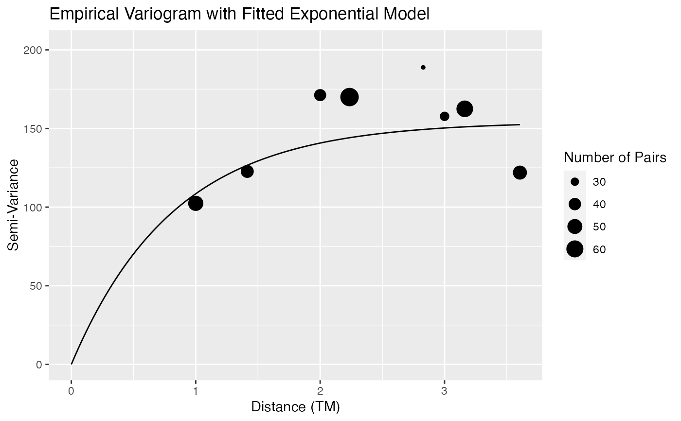
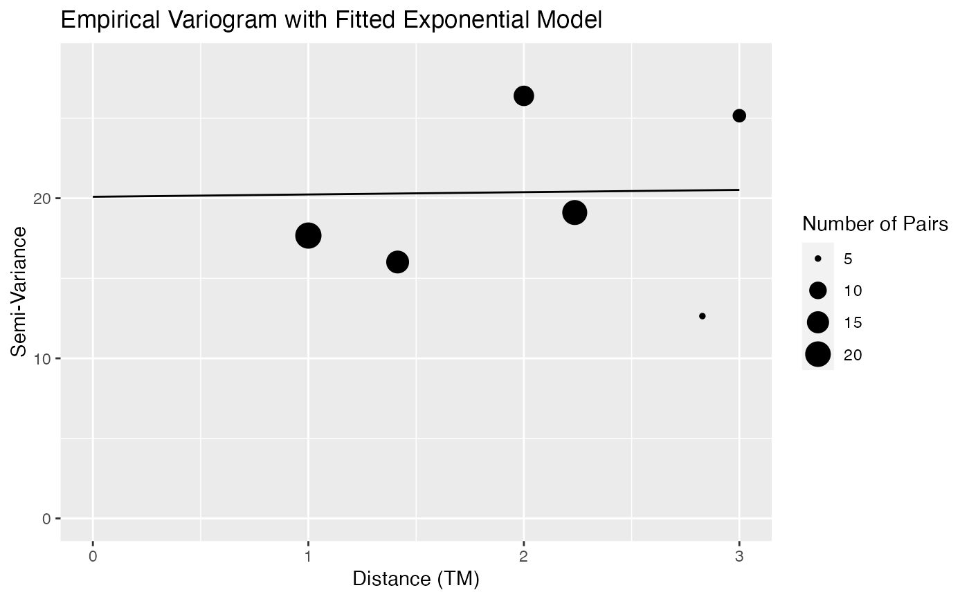
Plots an empirical semi-variogram of the residuals from the spatial linear model with the fitted parametric model as a curve overtop of the binned points. By default, the empirical semi-variogram only shows distances that are less than or equal to the maximum distance in the data set divided by 2. Therefore, it's possible that the REML-fitted model will not "fit" the points perfectly.
# S3 method for slmfit
plot(x, ...)
Arguments
- x
is an object of class
slmfit.- ...
further arguments passed to or from other methods.
Value
a plot of the empirical semi-variogram with the fitted model overlayed.
Examples
data(exampledataset) ## load a toy data set
slmobj <- slmfit(formula = counts ~ pred1 + pred2, data = exampledataset,
xcoordcol = 'xcoords', ycoordcol = 'ycoords', areacol = 'areavar')
plot(slmobj)


data(exampledataset) ## load a toy data set
exampledataset$strata <- c(rep("A", 19), rep("B", 21))
strataobj <- slmfit(formula = counts ~ pred1 + pred2, data = exampledataset, stratacol = "strata",
xcoordcol = 'xcoords', ycoordcol = 'ycoords', areacol = 'areavar')
plot(strataobj[[1]])
