Inference for Totals and Weighted Sums from Finite Spatial Populations

Introduction

The sptotal package was developed for predicting a weighted sum, most commonly a mean or total, from a finite number of sample units in a fixed geographic area. Estimating totals and means from a finite population is an important goal for both academic research and management of environmental data. One naturally turns to classical sampling methods, such as simple random sampling or stratified random sampling. Classical sampling methods depend on probability-based sample designs and are robust. Very few assumptions are required because the probability distribution for inference comes from the sample design, which is known and under our control. For design-based methods, sample plots are chosen at random, they are measured or counted, and inference is obtained from the probability of sampling those units randomly based on the design (e.g., Horwitz-Thompson estimation). As an alternative, we will use model-based methods, specifically geostatistics, to accomplish the same goals. Geostatistics does not rely on a specific sampling design. Instead, when using geostatistics, we assume the data were produced by a stochastic process with parameters that can be estimated. The relevant theory is given by Ver Hoef (2008). The sptotal package puts much of the code and plots in Ver Hoef (2008) in easily accessible, convenient functions.

In the sptotal package, our goal is to estimate some linear function of all of the sample units, call it $\tau(\mathbf{z}) = \mathbf{b}^\prime \mathbf{z}$, where $\mathbf{z}$ is a vector of the realized values for all the sample units and $\mathbf{b}$ is a vector of weights. By “realized,” we mean that whatever processes produced the data have already happened, and that, if we had enough resources, we could measure them all, obtaining a complete census. If $\tau(\mathbf{z})$ is a population total, then every element of $\mathbf{b}$ contains a $1$. Generally, $\mathbf{b}$ can contain any set of weights that we would like to multiply times each value in a population, and then these are summed, yielding a weighted sum.

The vector $\mathbf{b}$ contains the weights that we would apply if we could measure or count every observation, but, because of cost consideration, we usually only have a sample.

Data

Prior to using the sptotal package, the data needs to be in R in the proper format. For this package, we assume that your data set is a data.frame() object, described below.

Data Frame Structure

Data input for the sptotal package is a data.frame. The basic information required to fit a spatial linear model, and make predictions, are the response variable, covariates, the x- and y-coordinates, and a column of weights. You can envision your whole population of possible samples as a data.frame organized as follows,

where the red rectangle represents the column of the response variable, and the top part, colored in red, are observed locations, and the lower part, colored in white, are the unobserved values. To the right, colored in blue, are possibly several columns containing covariates thought to be predictive for the response value at each location. Covariates must be known for both observed and unobserved locations, and the covariates for unobserved locations are shown as pale blue below the darker blue covariates for observed locations above. It is also possible that there are no available covariates.

The data.frame must have x- and y-coordinates, and they are shown as two columns colored in green, with the coordinates for the unobserved locations shown as pale green below the darker green coordinates for the observed locations above. The data.frame can have a column of weights. If one is not provided, we assume a column of all ones so that the prediction is for the population total. The column of weights is purple, with weights for the observed locations a darker shade, above the lighter shade of purple representing weights for unsampled locations. Finally, the data.frame may contain columns that are not relevant to predicting the weighted sum. These columns are represented by the orange color, with the sampled locations a darker shade, above the unsampled locations with the lighter shade.

Of course, the data do not have to be in exactly this order, either in terms of rows or columns. Sampled and unsampled rows can be intermingled, and columns of response variable, covariates, coordinates, and weights can be also be intermingled. The figure above is an idealized graphic of the data. However, this figure helps envision how the data are used and illustrate the goal. We desire a weighted sum, where the weights (in the purple column) are multiplied with the response variable (red/white) column, and then summed. Because some of the response values are unknown (the white values in the response column), covariates and spatial information (obtained from the x- and y-coordinates) are used to predict the unobserved (white) values. The weights (purple) are then applied to both the observed response values (red), and the predicted response values (white), to obtain a weighted sum. Because we use predictions for unobserved response values, it is important to assess our uncertainty, and the software provides both an estimate of the weighted sum, mean, or total for the response variable as well as its estimated prediction variance.

Simulated Data Creation

To demonstrate the package, we created some simulated data so they are perfectly behaved, and we know exactly how they were produced. Here, we give a brief description before using the main features of the package. To get started, install the package

install.packages("sptotal")

and then type

library(sptotal)

Type

data(simdata)

and then simdata will be available in your workspace. To see the first six observations of simdata, type

head(simdata)
#>       x     y         X1          X2         X3          X4          X5
#> 1 0.025 0.975 -0.8460525  0.11866907 -0.2123901  0.38430607  0.08154129
#> 2 0.025 0.925 -0.6583116 -0.07686491 -0.9001410 -1.24774376  1.46631630
#> 3 0.025 0.875  0.2222961 -0.22803942  0.2820468  0.20560677  0.48713665
#> 4 0.025 0.825 -0.5433925  0.56894993 -0.9839629 -0.04950434 -0.78195604
#> 5 0.025 0.775 -0.7550155 -0.72592167 -0.4217208  0.26767033  0.40493269
#> 6 0.025 0.725 -0.1786784  0.33452155 -1.2134533  2.18704575 -0.54903128
#>           X6         X7 F1 F2        Z   wts1 wts2
#> 1  1.0747592 -0.0252824  3  3 15.94380 0.0025    0
#> 2  0.1299263  1.4651052  2  5 15.04616 0.0025    0
#> 3 -0.2537515  0.2682010  2  3 14.52765 0.0025    0
#> 4 -0.3259937  0.7858140  2  5 12.13401 0.0025    0
#> 5 -1.2284475  1.2944342  2  2 11.75260 0.0025    0
#> 6 -1.0366099  0.7938890  1  4 11.58142 0.0025    0

simdata is a data frame with 400 observations. The spatial coordinates are numeric variables in columns named x and y. We created 7 continuous covariates, X1 through X7. The variables X1 through X5 were all created using the rnorm() function, so they are all standard normal variates that are independent between and within variable. Variables X6 and X7 were independent from each other, but spatially autocorrelated within, each with a variance parameter of 1, an autocorrelation range parameter of 0.2 from an exponential model, and a small nugget effect of 0.01. The variables F1 and F2 are factor variables with 3 and 5 levels, respectively. The variable Z is the response. Data were simulated from the model

\[\begin{align*} Z_i = 10 & + 0 \cdot X1_i + 0.1 \cdot X2_i + 0.2 \cdot X3_i + 0.3 \cdot X4_i + \\ & 0.4 \cdot X5_i + 0.4 \cdot X6_i + 0.1 \cdot X7_i + F1_i + F2_i + \delta_i + \varepsilon_i \end{align*}\]

where factor levels for F1 have effects $0, 0.4, 0.8$, and factor levels for F2 have effects $0, 0.1, 0.2, 0.3, 0.4$. The random errors $\{\delta_i\}$ are spatially autocorrelated from an exponential model,

\[ \textrm{cov}(\delta_i,\delta_j) = 2*\exp(-d_{i,j}) \]

where $d_{i,j}$ is Euclidean distance between locations $i$ and $j$. In geostatistics terminology, this model has a partial sill of 2 and a range of 1. The random errors $\{\varepsilon_i\}$ are independent with variance 0.02, and this variance is called the nugget effect. Two columns with weights are included, wts1 contains 1/400 for each row, so the weighted sum will yield a prediction of the overall mean. The column wts2 contains a 1 for 25 locations, and 0 elsewhere, so the weighted sum will be a prediction of a total in the subset of 25 locations.

The spatial locations of simdata are in a $20 \times 20$ grid uniformly spaced in a box with sides of length 1,

require(ggplot2)
ggplot(data = simdata, aes(x = x, y = y)) + geom_point(size = 3) +
  geom_point(data = subset(simdata, wts2 == 1), colour = "red",
    size = 3)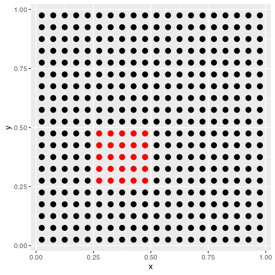

The locations of the 25 sites where wts2 is equal to one are shown in red.

We have simulated the data for the whole population. This is convenient, because we know the true means and totals. In order to compare with the prediction from the sptotal package, let’s find the true population total

sum(simdata[ ,'Z'])
#> [1] 4834.326

as well as the total in the subset of 25 sites

sum(simdata[ ,'wts2'] * simdata[ ,'Z'])
#> [1] 273.3751

However, we will now sample from this population to provide a more realistic setting where we can measure only a part of the whole population. In order to make results reproducible, we use the set.seed command, along with sample. The code below will replace some of the response values with NA to represent the unsampled sites.

set.seed(1)
# take a random sample of 100
obsID <- sample(1:nrow(simdata), 100)
simobs <- simdata
simobs$Z <- NA
simobs[obsID, 'Z'] <- simdata[obsID, 'Z']

We now have a data set where the whole population is known, simdata, and another one, simobs, where 75% of the response variable of the population has been replaced by NA. Next we show the sampled sites as solid circles, while the missing values are shown as open circles, and we use red again to show the sites within the small area of 25 locations.

ggplot(data = simobs, aes(x = x, y = y)) +
  geom_point(shape = 1, size = 2.5, stroke = 1.5) +
  geom_point(data = subset(simobs, !is.na(Z)), shape = 16, size = 3.5) +
  geom_point(data = subset(simobs, !is.na(Z) & wts2 == 1), shape = 16,
    colour = "red", size = 3.5) +
  geom_point(data = subset(simobs, is.na(Z) & wts2 == 1), shape = 1,
    colour = "red", size = 2.5, stroke = 1.5)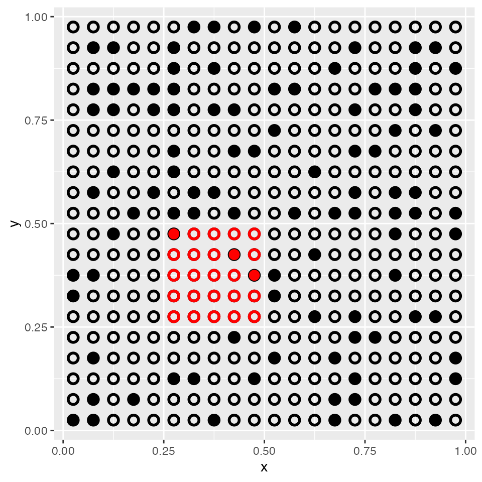

We will use the simobs data to illustrate use of the sptotal package.

Using the `sptotal` Package

After your data is in a similar format to simobs, using the sptotal package occurs in two primary stages. In the first, we fit a spatial linear model. This stage estimates spatial regression coefficients and spatial autocorrelation parameters. In the second stage, we predict the unsampled locations for the response value, and create a prediction for the weighted sum (e.g. the total) of all response variable values, both observed and predicted. To show how the package works, we demonstrate on ideal, simulated data. Then, we give a realistic example on moose data and a second example on lakes data to provide further insight and documentation. The moose example also has a section on data preparation steps.

Fitting a Spatial Linear Model: `slmfit`

We continue with our use of the simulated data, simobs, to illustrate fitting the spatial linear model. The spatial model-fitting function is slmfit (spatial-linear-model-fit), which uses a formula like many other model-fitting functions in R (e.g., the lm() function). To fit a basic spatial linear model we use

slmfit_out1 <- slmfit(formula = Z ~ X1 + X2 + X3 + X4 + X5 +
                        X6 + X7 + F1 + F2, 
                      data = simobs, xcoordcol = 'x',
                      ycoordcol = 'y',
                      CorModel = "Exponential")

The documentation describes the arguments in more detail, but as mentioned earlier, the linear model includes a formula argument, and the data.frame that is being used as a data set. We also need to include which columns contain the $x$- and $y$-coordinates, which are arguments to xcoordcol and ycoordcol, respectively. In the above example, we specify 'x' and 'y' as the column coordinates arguments since the names of the coordinate columns in our simulated data set are 'x' and 'y'. We also need to specify a spatial autocorrelation model, which is given by the CorModel argument. As with many other linear model fits, we can obtain a summary of the model fit,

summary(slmfit_out1)
#> 
#> Call:
#> Z ~ X1 + X2 + X3 + X4 + X5 + X6 + X7 + F1 + F2
#> 
#> Residuals:
#>     Min      1Q  Median      3Q     Max 
#> -1.9390 -0.6271  0.3338  1.2520  2.8137 
#> 
#> Coefficients:
#>             Estimate Std. Error t value Pr(>|t|)    
#> (Intercept) 11.36965    1.03775  10.956  < 2e-16 ***
#> X1          -0.05596    0.06400  -0.874  0.38437    
#> X2           0.02661    0.06606   0.403  0.68814    
#> X3           0.18292    0.06469   2.828  0.00583 ** 
#> X4           0.26487    0.05741   4.613    1e-05 ***
#> X5           0.38434    0.06022   6.382  < 2e-16 ***
#> X6           0.47612    0.11198   4.252    5e-05 ***
#> X7           0.02893    0.11761   0.246  0.80625    
#> F12          0.29596    0.15154   1.953  0.05407 .  
#> F13          0.70853    0.13136   5.394  < 2e-16 ***
#> F22          0.15384    0.17073   0.901  0.37008    
#> F23          0.19804    0.17828   1.111  0.26973    
#> F24          0.25492    0.20024   1.273  0.20641    
#> F25          0.39748    0.23691   1.678  0.09703 .  
#> ---
#> Signif. codes:  0 '***' 0.001 '**' 0.01 '*' 0.05 '.' 0.1 ' ' 1
#> 
#> Covariance Parameters:
#>              Exponential Model
#> Nugget            1.009265e-06
#> Partial Sill      2.930385e+00
#> Range             5.891474e-01
#> 
#> Generalized R-squared: 0.5996812

The output looks similar to the summary of a standard lm object, but there is some extra output at the end that gives our fitted covariance parameters. Plotting slmfit_out1 gives a semi-variogram of the residuals along with the fitted model:

plot(slmfit_out1)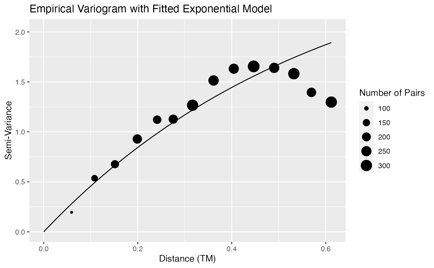

Note that the fitted curve may not appear to fit the empirical variogram perfectly for a couple of reasons. First, only pairs of points that have a distance between 0 and one-half the maximum distance are shown. Second, the fitted model is estimated using REML, which may give different results than using weighted least squares.

We can also examine a histogram of the residuals as well as a histogram of the cross-validation (leave-one-out) residuals:

residraw <- residuals(slmfit_out1)
qplot(residraw, bins = 20) + xlab("Residuals")
#> Warning: `qplot()` was deprecated in ggplot2 3.4.0.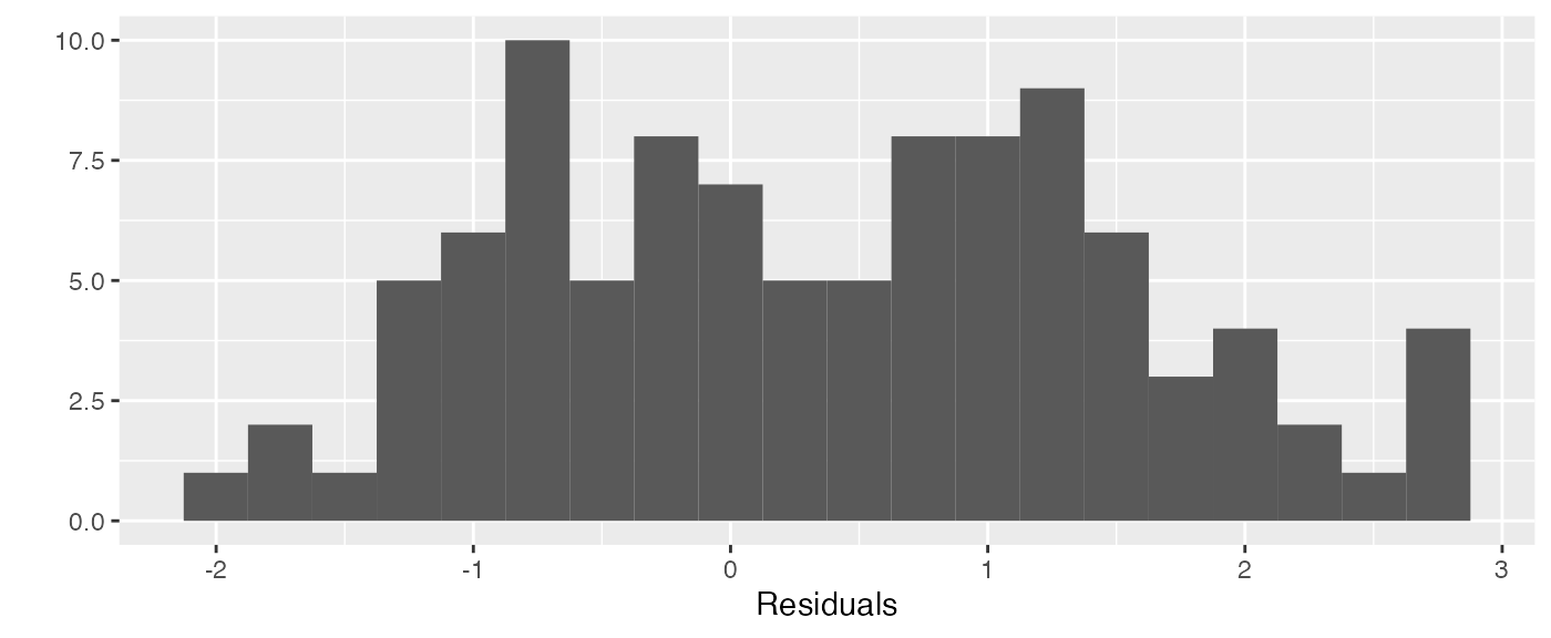

residcv <- residuals(slmfit_out1, cross.validation = TRUE)
qplot(residcv, bins = 20) + xlab("CV Residuals")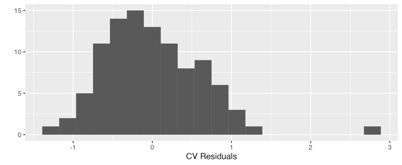

There is still one somewhat large cross-validation residual for an observed count that is larger than what would be predicted from a model without that particular count. The cause of this somewhat large residual can be attributed to random chance because we know that the data was simulated to follow all assumptions.

Prediction: `predict`

After we have obtained a fitted spatial linear model, we can use the predict() function to construct a data frame of predictions for the unsampled sites. By default, the predict() function assumes that we are predicting the population total and outputs this predicted total, the prediction variance for the total, a 90% prediction interval for the total, and some basic summary information about the number of sites sampled, the total number of units counted, etc. We name this object pred_obj in the chunk below and also construct a 90% confidence interval for the total.

pred_obj <- predict(slmfit_out1, conf_level = 0.90)
pred_obj

We predict a total of 4817 units in this simulated region with 90% confidence bounds of (4779, 4856). The prediction interval is fairly small because we simulated data that were highly correlated, increasing precision in prediction for unobserved sites. We can see that the prediction of the total is close to the true value of 4834.326, and the true value is within the prediction interval.

To access the data.frame that was input into slmfit, but is now appended with site-by-site predictions and site-by-site prediction variances, we can use pred_obj$Pred_df. This data set might be particularly useful if you would like to generate your own map with site-by-site predictions using other tools. The site-by-site predictions for density are given by the variable name_of_response_pred_density while the site-by-site predictions for counts are given by name_of_response_pred_count. These two columns will only differ if you have provided a column for areas of each site.

prediction_df <- pred_obj$Pred_df
head(prediction_df[ ,c("x", "y", "Z", "Z_pred_density")])

Examining results: `plot()`

Finally, to get a basic plot of the predictions, we can use the plot() function.

plot(pred_obj)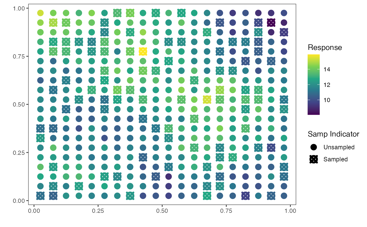

The map shows the distribution of the response across sampled and unsampled sites. Its purpose is simply to give the user a very quick idea of the distribution of the response. For example, we see from the plot that the predicted response is low in the upper-right region of the graph, is high in the middle of the region and in the upper-left corner of the region, and is low again at the lower portion of the area of interest. However, using the prediction data frame generated from the predict() function, you can use ggplot2 or any other plotting package to construct your own map that may be more useful in your context.

Prediction for a Small Area of Interest

Spatial prediction can be used to estimate means and totals over finite populations from geographic regions, but can also be used for the special case of estimating a mean or total in a small area of interest. The term small area estimation refers to making an inference on a smaller geographic area within the overall study area. There may be few or no samples within that small area, so that estimation by classical sampling methods may not be possible or variances become exceedingly large.

If we want to predict a quantity other than the population total, then we need to specify the column in our data set that has the appropriate prediction weights in a wtscol argument. For example, we might want to predict the total for a small area of interest. if we want to predict the total for the 25 sites in coloured in red, then we can use

pred_obj2 <- predict(slmfit_out1, wtscol = "wts2")
print(pred_obj2)
#> Prediction Info:
#>   Prediction    SE 90% LB 90% UB
#> Z      282.2 7.342  270.1  294.3
#>   Numb. Sites Sampled Total Numb. Sites Total Observed Average Density
#> Z                 100               400           1220            12.2

Recall that the true total for this small area was 273.4. We see that this is close to our prediction of 282.2 and is also within the bounds of our prediction interval.

Real Data Examples

Moose Abundance from Aerial Surveys

The simulated data example assumes that the coordinates are a Transverse Mercator projection (TM), that the vector of the response is numeric and has NA values for sites that were not sampled, and that the areas of each site sampled are all the same. For this example, we consider a data set on moose abundance in Alaska obtained from Alaska Department of Fish and Game, Division of Wildlife Conservation. Each observation corresponds to a moose counted at a particular site, but operational constraints do not permit all sites to be counted. We begin by loading the data into R.

data(AKmoose_df)

Some of the variables of interest include

total, which has counts of moose (and is NA for all sites that were not surveyed).
strat, a covariate that is either L for Low or M for medium.
surveyed, which is a 0 if the site wasn’t sampled and a 1 if the site was sampled.
x and y, the spatial coordinates for the centroids of the sites (in a user-defined Trans-Mercator projection).

Fitting the Model and Obtaining Predictions

We can now proceed to use the functions in sptotal in a similar way to how the functions were used for the simulated data. To get a sense of the data, we first give a plot of the raw observed counts:

ggplot(data = AKmoose_df, aes(x = x, y = y)) +
  geom_point(aes(colour = total), size = 4) +
  scale_colour_viridis_c() +
  theme_bw()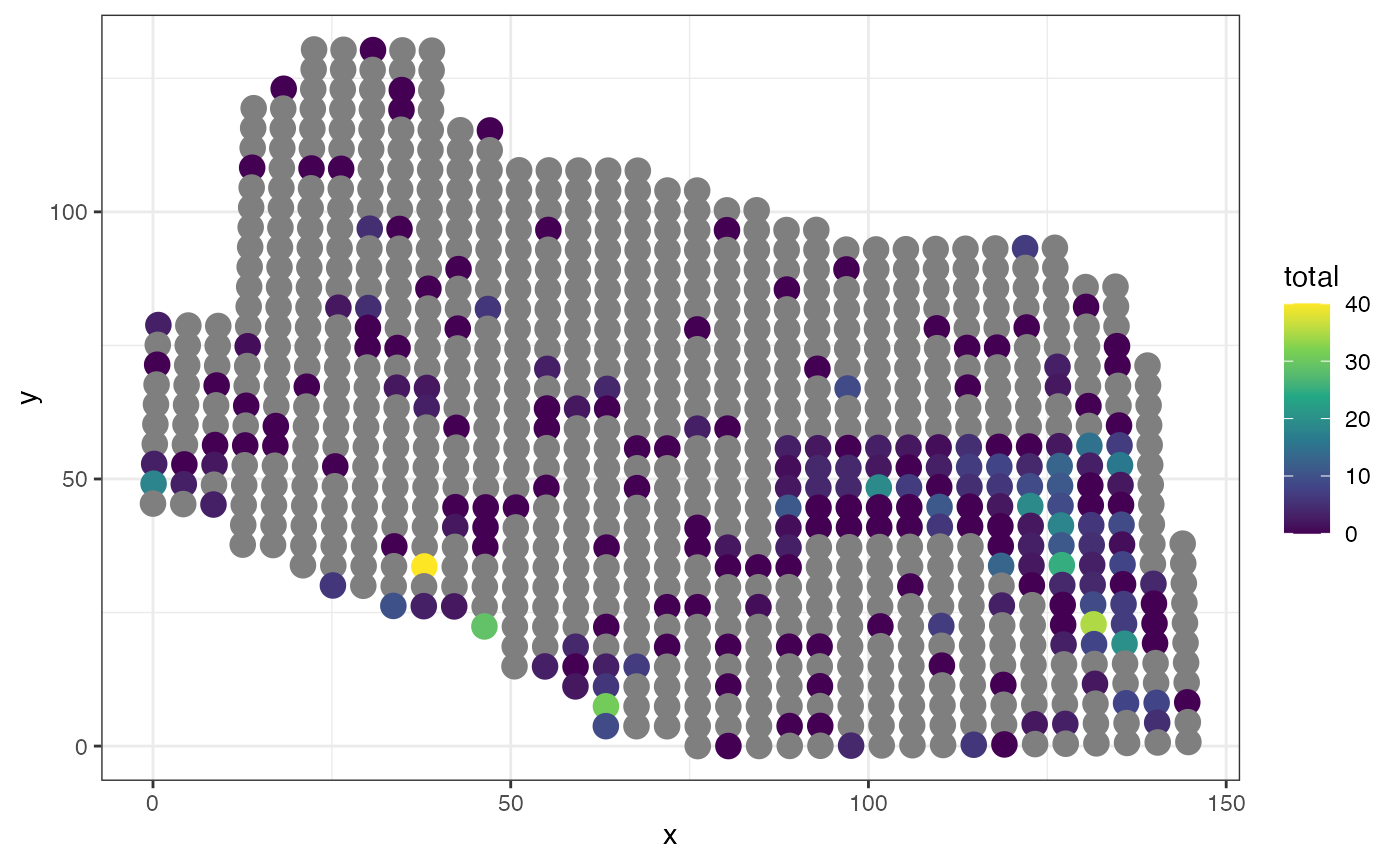

where the grey circles are sites that have not been sampled.

slmfit_out_moose <- slmfit(formula = total ~ strat, 
  data = AKmoose_df, xcoordcol = 'x', ycoordcol = 'y',
  CorModel = "Exponential")
summary(slmfit_out_moose)
plot(slmfit_out_moose)

resid_df <- data.frame(residuals = residuals(slmfit_out_moose,
                                             cross.validation = TRUE))
ggplot(data = resid_df, aes(x = residuals)) +
  geom_histogram(colour = "black", fill = "white", bins  = 20) +
  labs(x = "CV Residuals")

pred_moose <- predict(slmfit_out_moose)
pred_moose
plot(pred_moose)

We obtain a predicted total of 1596 animals with 90% lower and upper confidence bounds of 921 and 2271 animals, respectively. Unlike the simulation setting, there is no “true total” we can compare our prediction to, because, in reality, not all sites were sampled!

Allowing Different Covariance Parameters for Strata

Putting strat as a predictor in the model formula means that we are allowing each stratum to have a different mean but are assuming each stratum to have the same variance and covariance. If we want to allow the two strata to have different covariance parameter estimates, we can remove strat from the model formula and add it to the stratacol argument:

slmfit_out_moose_strat <- slmfit(formula = total ~ 1, 
  data = AKmoose_df, xcoordcol = 'x', ycoordcol = 'y',
  stratacol = "strat",
  CorModel = "Exponential")
summary(slmfit_out_moose_strat)
#> $L
#> 
#> Call:
#> total ~ 1
#> 
#> Residuals:
#>     Min      1Q  Median      3Q     Max 
#> -2.8337 -2.8337 -2.8337  0.1663 26.1663 
#> 
#> Coefficients:
#>      Estimate Std. Error t value Pr(>|t|)
#> [1,]    2.834      2.076   1.365    0.176
#> 
#> Covariance Parameters:
#>              Exponential Model
#> Nugget                6.548489
#> Partial Sill         23.421310
#> Range                32.274509
#> 
#> Generalized R-squared: 2.220446e-16 
#> 
#> $M
#> 
#> Call:
#> total ~ 1
#> 
#> Residuals:
#>     Min      1Q  Median      3Q     Max 
#> -4.0571 -4.0571 -2.0571  0.9429 35.9429 
#> 
#> Coefficients:
#>      Estimate Std. Error t value Pr(>|t|)  
#> [1,]    4.057      1.838   2.207    0.029 *
#> ---
#> Signif. codes:  0 '***' 0.001 '**' 0.01 '*' 0.05 '.' 0.1 ' ' 1
#> 
#> Covariance Parameters:
#>              Exponential Model
#> Nugget                37.62337
#> Partial Sill          12.12722
#> Range                 37.68748
#> 
#> Generalized R-squared: 0

There is now two sets of summary output, one for each stratum. predict() can still be used to obtain an estimate for the total (predict() also gives a predicted total for each stratum):

predict(slmfit_out_moose_strat)
#> 
#> Prediction and Confidence Intervals:
#>       Prediction    SE 90% LB 90% UB
#> L         1133.4 303.2  634.6   1632
#> M          960.8 104.3  789.2   1132
#> Total     2094.2 320.7 1566.8   2622

For this example, our prediction is very different when strata are allowed separate covariance parameters (2094 moose) than when strata are forced to have the same covariance parameters (1596 moose).

To see why this is, we can examine the semi-variograms for each stratum. All functions (e.g. plot(), AIC(), coef(), etc.) that are used on an slmfit() object without stratacol specified can still be used on an slmfit() object with a stratacol specified by running the function in the following way:

plot(slmfit_out_moose_strat[[1]])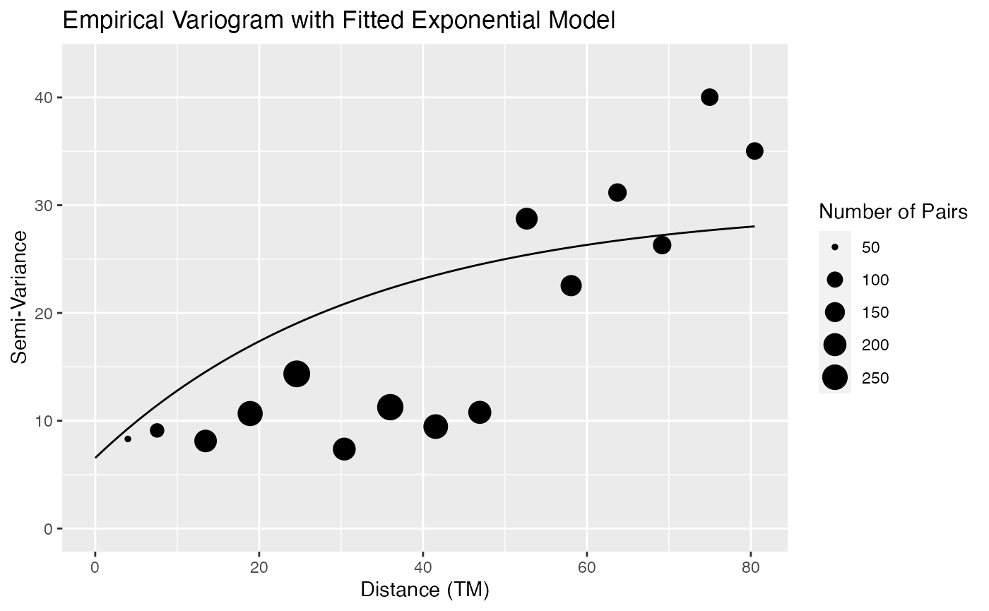

plot(slmfit_out_moose_strat[[2]])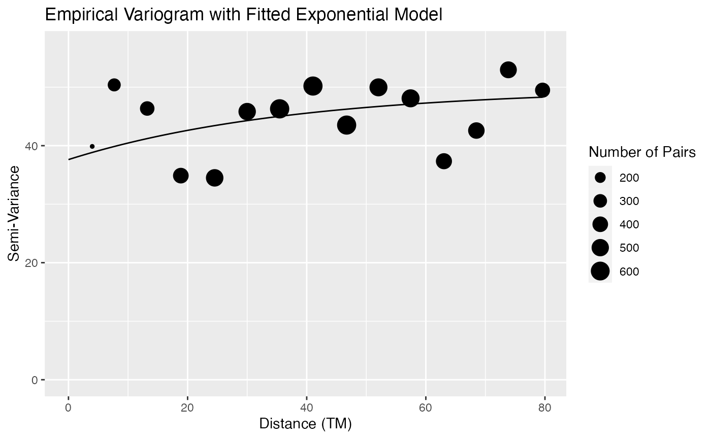

We see that the fitted covariance parameters for each strata do look different in this example, as the scale on the semi-variograms changes drastically. Therefore, for this example, it is probably more reasonable to allow the strata to have different covariance parameters and use the stratacol argument.

Sites with Different Areas

Finally, throughout all of the above analyses, we have assumed that the areas of each site were equal. Though this assumption is not accurate for the moose data, due to slightly differing areas based on differing latitudes and longitudes, the assumption approximately holds so that any differences in the prediction that incorporates area is negligible. But, suppose we had sites with very different areas. To showcase how to incorporate site area into the functions in this package, let’s first create a “fake” area variable that has the first 700 sites in the region have an area of 1 square kilometer and has the last 160 sites in the region have an area of 2 square kilometers.

AKmoose_df$fake_area <- c(rep(1, 700), rep(2, 160))

For a spatial model, it makes much more sense to use density as the response variable instead of raw counts if the areas of the sites in the model are drastically different. By supplying an areacol argument to slmfit, the function converts counts to densities, and then gives regression parameters and covariance parameters for the density.

slmfit_out_moose_area <- slmfit(formula = total ~ strat, 
  data = AKmoose_df, xcoordcol = 'x', ycoordcol = 'y',
  CorModel = "Exponential", areacol = 'fake_area')
summary(slmfit_out_moose_area)
#> 
#> Call:
#> total ~ strat
#> 
#> Residuals:
#>     Min      1Q  Median      3Q     Max 
#> -3.3072 -3.3072 -1.0906  0.9094 36.6928 
#> 
#> Coefficients:
#>             Estimate Std. Error t value Pr(>|t|)   
#> (Intercept)   1.0906     0.9138   1.193  0.23401   
#> stratM        2.2166     0.6964   3.183  0.00167 **
#> ---
#> Signif. codes:  0 '***' 0.001 '**' 0.01 '*' 0.05 '.' 0.1 ' ' 1
#> 
#> Covariance Parameters:
#>              Exponential Model
#> Nugget               20.711292
#> Partial Sill          4.166747
#> Range                23.645337
#> 
#> Generalized R-squared: 0.04479698

The predict function then keeps track of the areacol argument and gives output in the data frame that pertains to both counts and densities:

pred_obj_area <- predict(slmfit_out_moose_area)
head(pred_obj_area$Pred_df[ ,c("total_pred_density", "total_pred_count",
                               "fake_area")])
#>   total_pred_density total_pred_count fake_area
#> 0          0.4029168        0.4029168         1
#> 1          0.3505312        0.3505312         1
#> 2          0.0000000        0.0000000         1
#> 3          0.2841390        0.2841390         1
#> 4          0.2782489        0.2782489         1
#> 5          0.3290719        0.3290719         1
tail(pred_obj_area$Pred_df[ ,c("total_pred_density", "total_pred_count",
                               "fake_area")])
#>     total_pred_density total_pred_count fake_area
#> 854         2.00000000       4.00000000         2
#> 855         0.01496504       0.02993008         2
#> 856         0.02163868       0.04327737         2
#> 857         0.06967022       0.13934044         2
#> 858         0.00000000       0.00000000         2
#> 859         0.49928987       0.99857974         2

Note that, for the first 6 observations, which have an area of 1, the total_pred_density and total_pred_count columns are identical, while, for the last 6 observations, which have an area of 2, the total_pred_density column is half that of the total_pred_count column.

Because we did not specify a column of weights, our prediction in the following output is for the total number of moose.

print(pred_obj_area)
#> Prediction Info:
#>       Prediction    SE 90% LB 90% UB
#> total       1556 393.6    909   2204
#>       Numb. Sites Sampled Total Numb. Sites Total Observed Average Density
#> total                 218               860            742           2.883

If sites have differing areas, the plot() function doesn’t make much sense to use because each site is represented by the same-sized dot. Here, it would be helpful to import the data frame with the predicted counts and densities into a shapefile so that you are able to construct your own graphics that reflect the different-sized sites.

Mean Dissolved Organic Carbon from National Lakes Data

As another example, we took data from the National Aquatic Resource Surveys. With concerns about global warming, the earth’s capacity to store carbon is of great interest, and dissolved organic carbon (DOC) is an estimate of a lake’s ability to store carbon. We will estimate the mean mg/L for DOC from a sample of lakes. If the total lake volume could be calculated (we will not attempt that), then the total dissolved carbon in a population of lakes could be estimated. We will examine DOC in lakes from the 2012 surveys. We combined site data, DOC data, and habitat metrics to create a data set of 1206 lakes in the conterminous United States.

To access the data, type

data(USlakes)

and create a histogram of the log dissolved organic carbon

ggplot(data = USlakes, aes(x = log(DOC_RESULT))) +
  geom_histogram(bins = 20)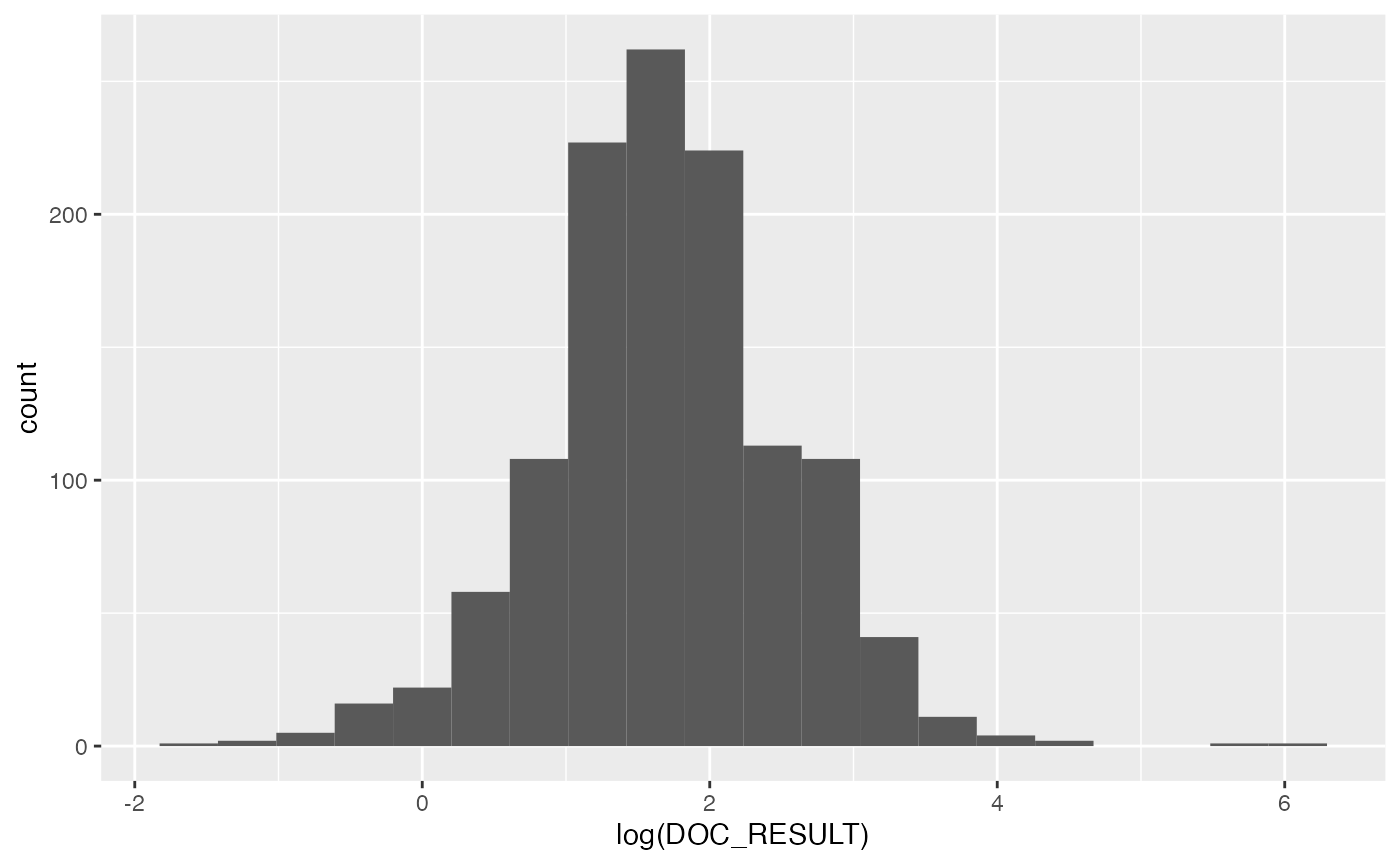

Even on the log scale, there appears to be some outliers with very high values, and these may be the result of errors in collection or lab analysis. We will eliminate lakes that have log(DOC) values $>$ 5 for the purposes of this vignette.

lakes <- USlakes[log(USlakes$DOC_RESULT) < 5, ]

Our new data set has

nrow(lakes)
#> [1] 1204

sites, so we have eliminated 2 sites. To visualize our data more, we make a bubble plot,

plot(USlakes$XCOORD, USlakes$YCOORD, pch = 19, 
  cex = 2 * log(lakes$DOC_RESULT) / max(log(lakes$DOC_RESULT)))

and it appears that there is spatial patterning.

We also have covariates that may help in prediction:

ELEVATION: Elevation at lake coordinates (LAT_DD_N83, LON_DD_N83) from NHD Digital Elevation Map layer
RVFPUNDWOODY_RIP: riparian zone and vegetation: fraction of understory with nonwoody cover present in the riparian zone
FCIBIG_LIT: Fish cover: index of fish cover due to large structures in the littoral zone
RVFCGNDBARE_RIP: riparian zone and vegetation: fraction of ground lacking cover in the riparian zone
RVFCGNDWOODY_RIP: riparian zone and vegetation: fraction of ground cover by woody vegetation in the riparian zone

In order to explore the association between each predictor and the DOC (but not yet taking into account spatial correlation), we would create scatterplots of DOC vs. each predictor. To save space, we only create one such scatterplot here:

ggplot(data = lakes,
       aes(x = RVFPUNDWOODY_RIP, y = log(DOC_RESULT))) +
  geom_jitter(width = 0.02) +
  geom_smooth(method = "lm", se = TRUE)
#> `geom_smooth()` using formula = 'y ~ x'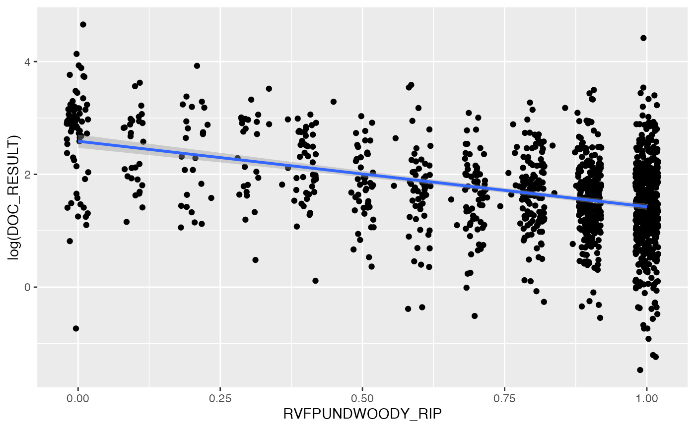

It looks like there might be a slight negative relationship between riparian nonwoody-understory cover and DOC, though again we note that this exploratory investigation does not take into account the possible spatial correlation of DOC across sites.

Creating a Subsample Data Set

We have the whole population of lakes, but, with budget cuts, it is likely that this whole population will not always be surveyed in its entirety. So, we will ask the question, “If we sample from this population, can we still get a fairly precise estimate of the mean DOC?”

We will do the same thing that we did with the simulated data, and take a random sample of 500 lakes. Also, because we want the mean, and not a total, we will create a weights column for the lakeobs data set, with each element $1/N$, where, here, $N = 1204$.

set.seed(2)
LakeObsID <- sample(1:nrow(lakes), 500)
lakeobs <- lakes
lakeobs$DOC_RESULT <- NA
lakeobs[LakeObsID, 'DOC_RESULT'] <- lakes[LakeObsID, 'DOC_RESULT']
lakeobs$wts <- 1 / nrow(lakeobs)

Fitting the Model and Making Predictions

Even though data are skewed, let’s try it without taking log of response variable. Note that the mean of log-transformed variables is not equal to the log of the mean of set of variables. So if we want a total on the untransformed scale, it would be a mistake to transform the data first, model it, make predictions, sum the predictions, and then exponentiate. It is much simpler to leave the data untransformed and rely on robustness of the method. Let’s see how this works.

slmfitout_exp_lakes <- slmfit(formula = DOC_RESULT ~ ELEVATION +
                                RVFPUNDWOODY_RIP + FCIBIG_LIT +
                                RVFCGNDBARE_RIP + RVFCGNDWOODY_RIP,
                              data = lakeobs, 
                              xcoordcol = 'XCOORD', ycoordcol = 'YCOORD', CorModel = "Exponential")
summary(slmfitout_exp_lakes)
#> 
#> Call:
#> DOC_RESULT ~ ELEVATION + RVFPUNDWOODY_RIP + FCIBIG_LIT + RVFCGNDBARE_RIP + 
#>     RVFCGNDWOODY_RIP
#> 
#> Residuals:
#>      Min       1Q   Median       3Q      Max 
#> -14.4226  -6.1203  -4.2384  -0.6852  88.0354 
#> 
#> Coefficients:
#>                    Estimate Std. Error t value Pr(>|t|)    
#> (Intercept)      18.5585533  2.8978665   6.404  < 2e-16 ***
#> ELEVATION        -0.0015922  0.0009541  -1.669  0.09579 .  
#> RVFPUNDWOODY_RIP -7.7307967  1.2430529  -6.219  < 2e-16 ***
#> FCIBIG_LIT       -4.0559783  1.6831386  -2.410  0.01633 *  
#> RVFCGNDBARE_RIP  -4.4469366  1.6693922  -2.664  0.00798 ** 
#> RVFCGNDWOODY_RIP  1.1457813  1.7641454   0.649  0.51633    
#> ---
#> Signif. codes:  0 '***' 0.001 '**' 0.01 '*' 0.05 '.' 0.1 ' ' 1
#> 
#> Covariance Parameters:
#>              Exponential Model
#> Nugget                15.09434
#> Partial Sill          91.02786
#> Range             456983.39560
#> 
#> Generalized R-squared: 0.1188291

We see that all covariates are highly significant. There is substantial autocorrelation because the range parameter is very large, and the partial sill is about six times that of the nugget effect. We fit the model again, but this time with the spherical autocorrelation model.

slmfitout_sph_lakes <- slmfit(formula = DOC_RESULT ~ ELEVATION +
                                RVFPUNDWOODY_RIP + FCIBIG_LIT +
                                RVFCGNDBARE_RIP + RVFCGNDWOODY_RIP,
                              data = lakeobs, 
                              xcoordcol = 'XCOORD', ycoordcol = 'YCOORD',
                              CorModel = "Spherical")
summary(slmfitout_sph_lakes)
#> 
#> Call:
#> DOC_RESULT ~ ELEVATION + RVFPUNDWOODY_RIP + FCIBIG_LIT + RVFCGNDBARE_RIP + 
#>     RVFCGNDWOODY_RIP
#> 
#> Residuals:
#>      Min       1Q   Median       3Q      Max 
#> -13.5767  -5.5804  -3.6468  -0.1512  88.6358 
#> 
#> Coefficients:
#>                    Estimate Std. Error t value Pr(>|t|)    
#> (Intercept)      17.7013675  2.0458144   8.652  < 2e-16 ***
#> ELEVATION        -0.0012000  0.0009266  -1.295  0.19589    
#> RVFPUNDWOODY_RIP -7.7512748  1.2399212  -6.251  < 2e-16 ***
#> FCIBIG_LIT       -3.7733882  1.6698727  -2.260  0.02428 *  
#> RVFCGNDBARE_RIP  -4.3820168  1.6562157  -2.646  0.00841 ** 
#> RVFCGNDWOODY_RIP  1.3173261  1.7526027   0.752  0.45263    
#> ---
#> Signif. codes:  0 '***' 0.001 '**' 0.01 '*' 0.05 '.' 0.1 ' ' 1
#> 
#> Covariance Parameters:
#>              Spherical Model
#> Nugget              15.74324
#> Partial Sill        87.85260
#> Range           761505.47106
#> 
#> Generalized R-squared: 0.1151265

We can use AIC to compare the use of the two autocorrelation models.

AIC(slmfitout_exp_lakes)
#> [1] 3249.515
AIC(slmfitout_sph_lakes)
#> [1] 3248.077

Based on AIC, there is not much difference in fit between the two structures. We will use the exponential covariance structure going forward.

pred_exp_lakes <- predict(slmfitout_exp_lakes,  wtscol = "wts",
                          conf_level = 0.95)
print(pred_exp_lakes)
#> Prediction Info:
#>            Prediction    SE 95% LB 95% UB
#> DOC_RESULT      7.975 0.196  7.591  8.359
#>            Numb. Sites Sampled Total Numb. Sites Total Observed Average Density
#> DOC_RESULT                 500              1204           4111           8.223
mean(lakes$DOC_RESULT)
#> [1] 7.646453

We can see that the prediction, 7.975, is close to the true value, 7.65, and that the confidence interval is quite narrow, and it does contain the true value. If a standard error of 0.196, yielding a coefficient of variation of 0.196/7.975 = 0.0245, is acceptable, then sampling 500 lakes could save money and still provide a useful result on DOC.

Appendix: Statistical Background

An alternative to a sampling-based approach is to assume that the data were generated by a stochastic process and use model-based approaches. It is assumed that the response variable is a realization of a spatial stochastic process. Geostatistical models and methods are used (for a review, see Cressie, 1993). Geostatistics was developed for point samples. If the samples are very small relative to the population size, an infinite population is assumed. In classical geostatistics, the average value over an area can be predicted using methods such as block kriging. Thus it appears that this is closely related to small area estimation, but where samples come from point locations rather than a finite set of sample units. While there is a large literature on geostatistics and block kriging methods, they have been developed for infinite populations. This package is designed for the case where we have a finite collection of plots and we assume that the data were produced by a spatial stochastic process. Detailed developments are given in Ver Hoef (2001, 2008). Comparisons to classical sampling methods can be found in Ver Hoef (2002), and applications in forestry are contained in Ver Hoef and Temesgen (2013) and Temesgen and Ver Hoef (2015).

Citation

To cite this package, type

citation("sptotal")

References

Cressie, N. 1993. Statistics for Spatial Data, Revised Edition John Wiley and Sons, NY.

Temesgen, H. and Ver Hoef, J.M. 2015. Evaluation of the Spatial Linear Model, Random Forest and Gradient Nearest-Neighbour Methods for Imputing Potential Pro- ductivity and Biomass of the Pacific Northwest Forests. Forestry 88(1): 131–142.

Ver Hoef, J.M. 2001. Predicting Finite Populations from Spatially Correlated Data. 2000 Proceedings of the Section on Statistics and the Environment of the American Statistical Association, pgs. 93 – 98.

Ver Hoef, J.M. 2002. Sampling and Geostatistics for Spatial Data. Ecoscience 9: 152–161.

Ver Hoef, J. M. 2008. Spatial Methods for Plot-Based Sampling of Wildlife Populations. Environmental and Ecological Statistics 15: 3-13.

Ver Hoef, J.M. and Temesgen, H. 2013. A Comparison of the Spatial Linear Model to Nearest Neighbor (k-NN) Methods for Forestry Applications. PloS ONE 8(3): e59129.

Matt Higham, Jay M. Ver Hoef, Bryce M. Frank, Michael Dumelle

2023-02-01

Introduction

Data

Data Frame Structure

Simulated Data Creation

Using the `sptotal` Package

Fitting a Spatial Linear Model: `slmfit`

Prediction: `predict`

Examining results: `plot()`

Prediction for a Small Area of Interest

Real Data Examples

Moose Abundance from Aerial Surveys

Fitting the Model and Obtaining Predictions

Allowing Different Covariance Parameters for Strata

Sites with Different Areas

Mean Dissolved Organic Carbon from National Lakes Data

Creating a Subsample Data Set

Fitting the Model and Making Predictions

Appendix: Statistical Background

Citation

References

Inference for Totals and Weighted Sums from Finite Spatial Populations

Matt Higham, Jay M. Ver Hoef, Bryce M. Frank, Michael Dumelle

2023-02-01

Introduction

Data

Data Frame Structure

Simulated Data Creation

Using the sptotal Package

Fitting a Spatial Linear Model: slmfit

Prediction: predict

Examining results: plot()

Prediction for a Small Area of Interest

Real Data Examples

Moose Abundance from Aerial Surveys

Fitting the Model and Obtaining Predictions

Allowing Different Covariance Parameters for Strata

Sites with Different Areas

Mean Dissolved Organic Carbon from National Lakes Data

Creating a Subsample Data Set

Fitting the Model and Making Predictions

Appendix: Statistical Background

Citation

References

Using the `sptotal` Package

Fitting a Spatial Linear Model: `slmfit`

Prediction: `predict`

Examining results: `plot()`