Using the GSPE R Package

Introduction

The purpose of this vignette is to illustrate how to use the GSPE R Package for moose survey data, both with and without a separate sightability study. There are three primary sections, each building off the previous section. Throughout the Vignette, a simulated moose survey is used as an example. Though some of the documentation references moose specifically, the package can be used for many ecological studies with count data collected on a finite number of sites.

Section 1 shows how to obtain a population prediction assuming perfect detection.
Section 2 shows how to obtain a population prediction assuming constant detection across all sites.
Section 3 shows how to obtain a population prediction using radiocollar data with the possibility of site covariates useful for predicting detection.

Section 1: Perfect Detection

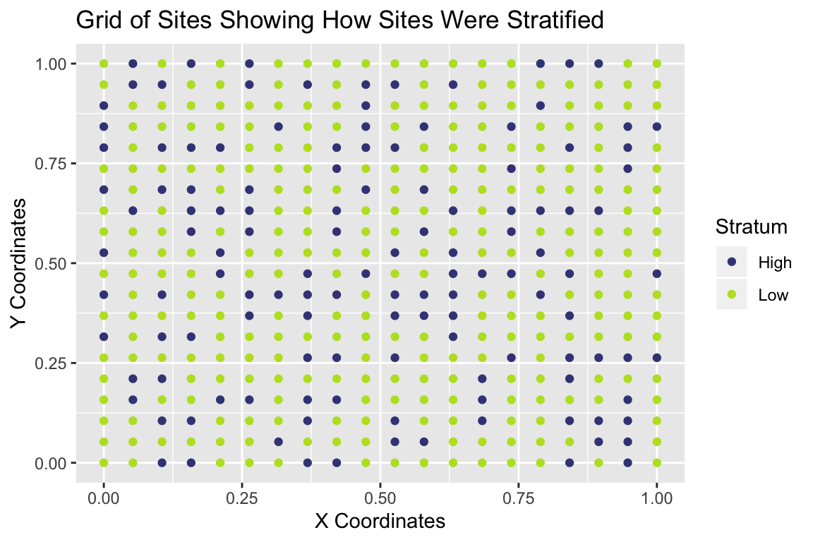
As mentioned above, we will use a simulated moose survey. Though we have sightability trials for this particular data set, suppose first that we want to assume perfect detection. Like many moose data sets, the sites are stratified into a “High” strata and a “Low” strata. Let’s load the FPBKPack2 library and take a look at the data set and at an accompanying map of the stratification.

The easiest way to install the package from GitHub is to use the install_git function in the devtools library.

## install the package first with devtools
## install.packages("devtools")

## devtools::install_git("https://github.com/highamm/FPBKPack2.git")
library(FPBKPack2)

simdf <- vignettecount

pander::pander(head(simdf[ ,c("Xcoords", "Ycoords", "Moose",
  "CountPred", "Stratum")]))

Xcoords	Ycoords	Moose	CountPred	Stratum
0.3158	0.3158	9	4.302	Low
0.7895	0.1579	23	1.901	Low
0.8947	0.1579	NA	2.507	Low
1	0	NA	2.521	Low
0.9474	0.5263	0	3.693	Low
0.3684	0.1053	NA	3.086	High

The title of the data set is simdf.

One aspect of the data set to note is that all of the counts on unsampled sites are given as NA values. By default, if uploading an Excel spreadsheet or a .csv file into R, any blank cells are converted to NA values. So, unsampled sites should have NA count values (not -9999 or NotSampled, etc.) before using the package functions.

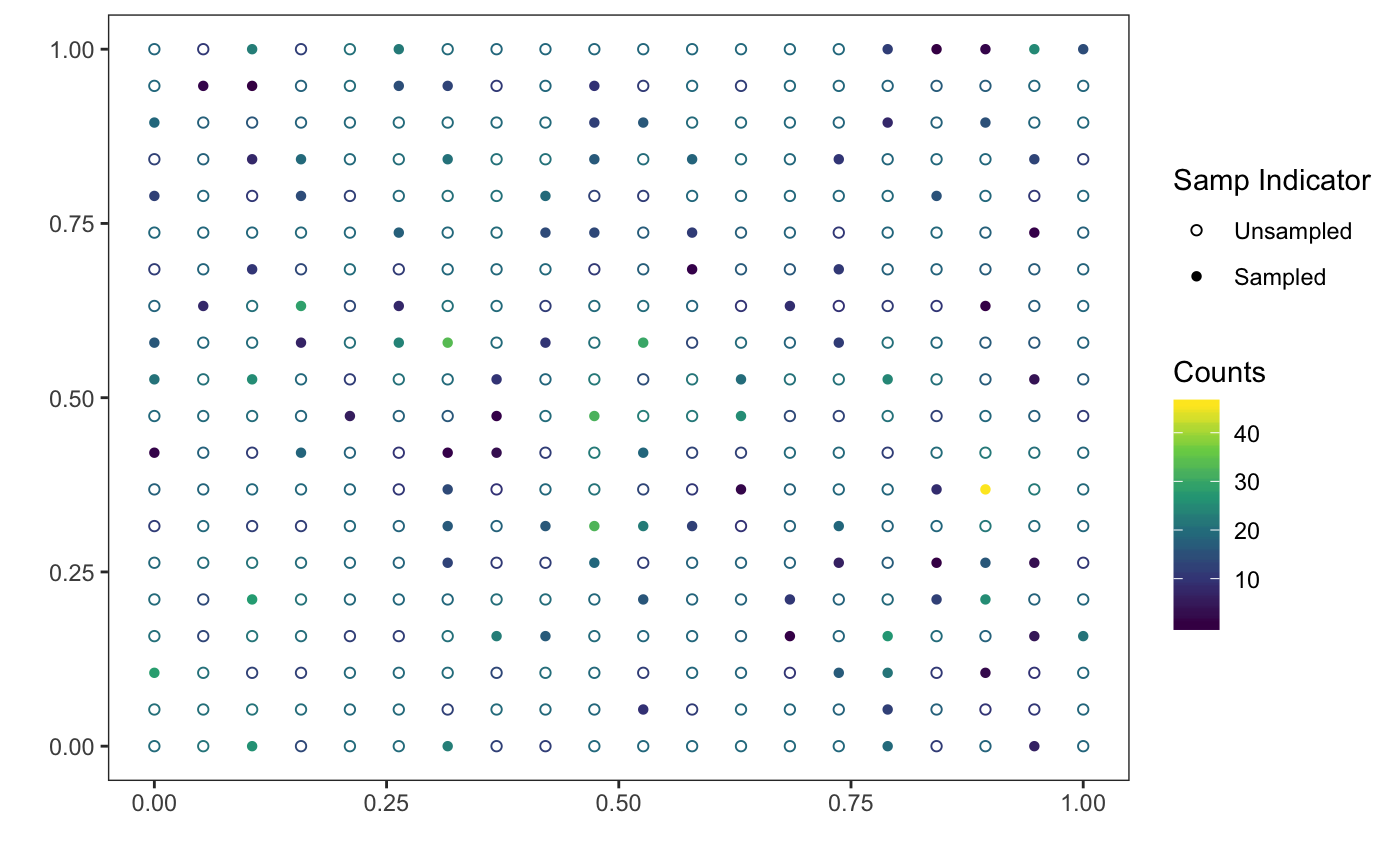
We can also look at a map of where sites were sampled:

library(ggplot2)

#minxdist <- min(dist(simdf$Xcoords)[dist(simdf$Ycoords) != 0])
#minydist <- min(dist(simdf$Xcoords)[dist(simdf$Ycoords) != 0])
simdf$samplingindicator <- factor(is.na(simdf$Moose))
levels(simdf$samplingindicator)[1] <- "Sampled"
levels(simdf$samplingindicator)[2] <- "Unsampled"

p3 <- ggplot(data = simdf, aes(x = Xcoords, y = Ycoords,
  colour = as.factor(samplingindicator))) +
  scale_colour_viridis_d("Sampling Indicator", begin = 0.2,
    end = 0.9) +
  geom_point() +
  xlab("X Coordinates") + ylab("Y Coordinates") +
  ggtitle("Grid of Sites Showing Which Were Sampled")
print(p3)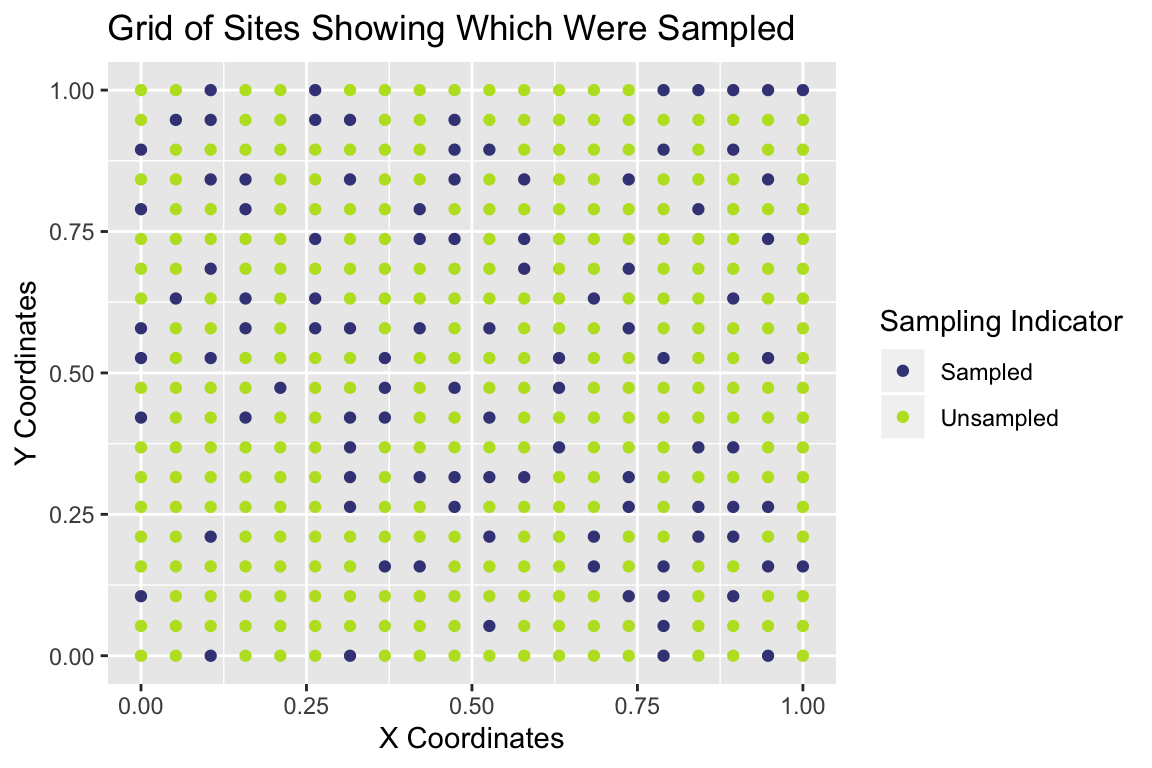

Stratifiacation

And we can examine a grid of the stratification structure:

R Shiny App

Much of the functionality of this package will be made available in an R Shiny app to be developed before the end of summer of 2019. The following Vignette shows how to use the package in R or RStudio directly. See the Shiny vignette if interested in using the package through the Shiny app.

Package Functions

There are five main functions that a user would call to obtain the population prediction. They are:

slmfit(Spatial Linear Model fit), used to fit covariance parameter estimates and obtain estimated regression coefficients,
predict, used to do the spatial prediction,
FPBKoutput to format the results,
multistrat to combine slmfit, predict, and FPBKoutput when fitting the model to multiple strata, and
get_reportdoc to obtain a report similar to the Winfonet report.

Most of the remainder of the functions in the package are helper functions called within the four main functions above.

The `slmfit` Function

slmfit has the most user inputs, including:

formula, an R formula in the form response ~ predictor1 + predictor2 + ...
data, the full data set containing both sampled and unsampled observations, including the predictors, the response, and the spatial coordinates.
xcoordcol, the name of the column containing x-coordinates, in quotes.
ycoordcol, the name of the column containing y-coordinates, in quotes.
CorModel, the covariance structure, defaulting to "Exponential" with "Gaussian" and "Spherical" as other possiblities.
areacol, the name of the column with site areas. If omitted, sites are assumed to have equal area.
coordtype, either TM by default which results in the package not modifying the coordinates or LatLon for latitude / longitude coordinates which results in conversion to TM coordinates within the package.
a few other optional arguments.

The formula input allows the user to put in categorical or continuous covariates that are thought to be associated with site count totals (eg. habitat covariates). For the Togiak March analysis, we do not have any such covariates so the formula used is response ~ 1. Throughout the package, we try to keep as much of the syntax as similar as possible to R’s lm function in the hopes that a new user already familiar with lm can more easily use the package.

Let’s first begin by obtaining a prediction for the population total in the high stratum. For this data set, the coordinates have already been converted from Latitude/Longitude coordinates into TM coordinates. For the simulated data set, the input would look like:

highdf <- subset(simdf, Stratum == "High")
slmobj <- slmfit(formula = Moose ~ 1,
  data = highdf,
  xcoordcol = "Xcoords",
  ycoordcol = "Ycoords",
  CorModel = "Exponential",
  areacol = "Area")

The slmobj has a lot of information within it. We can use the summary function to obtain some of the most pertinent information.

summary(slmobj)
#> 
#> Call:
#> Moose ~ 1
#> 
#> Residuals:
#>     Min      1Q  Median      3Q     Max 
#> -3.8975 -3.0225  0.1025  2.7275  8.6025 
#> 
#> Coefficients:
#>      Estimate Std. Error t value Pr(>|t|)    
#> [1,]   3.8975     0.9999   3.898  0.00025 ***
#> ---
#> Signif. codes:  0 '***' 0.001 '**' 0.01 '*' 0.05 '.' 0.1 ' ' 1
#> 
#> Covariance Parameters:
#>              Exponential Model
#> Nugget                10.60941
#> Partial Sill       74912.62873
#> Range              37324.30856

When areacol is included, then the spatial prediction utilizes densities, not counts. So, the coefficient estimate is the estimate the mean density in the high stratum. The densities are transformed back to counts in the predict function, which is described next.

The `predict` Function

The user then inputs the object created by slmfit to the predict function. The predict function has the following arguments:

object, a named model object from slmfit.
FPBKcol, the name of the column in the data set with prediction weights. If omitted, the predict function predicts the population total.
a few other arguments.

predobj <- predict(object = slmobj)

I’ve left the FPBKcol out for this example, resulting in a prediction for the population total. The predict function contains the prediction for the population total, the prediction variance, and the data set that the user input to slmfit with the following columns appended:

response_pred, the site-by-site predictions.
response_predvar, the site-by-site prediction variances.
response_sampind, an indicator column of which sites were sampled.
response_muhat, a column of means for the density at each site.

Some of these features are summarized in the following output function that generates a mini-report. However, having the appended data set available to the user can be beneficial to anyone who might want to obtain their own specific summary statistics, graphics, etc. using R or other software like GIS.

The `FPBKoutput` Function

The user can run the FPBKoutput function (Finite Population Block Kriging output). I’ve tried to structure much of the report output to be as similar to the WinfoNet output as possible. If using the package through the future R Shiny app, this report is output from the app in addition to a .csv file with the data set from predict. Inputs to FPBKoutput include:

pred_info, the object generated from predict.
conf_level, the desired confidence level for prediction intervals. By default, the output returns 80%, 90%, and 95% prediction intervals.
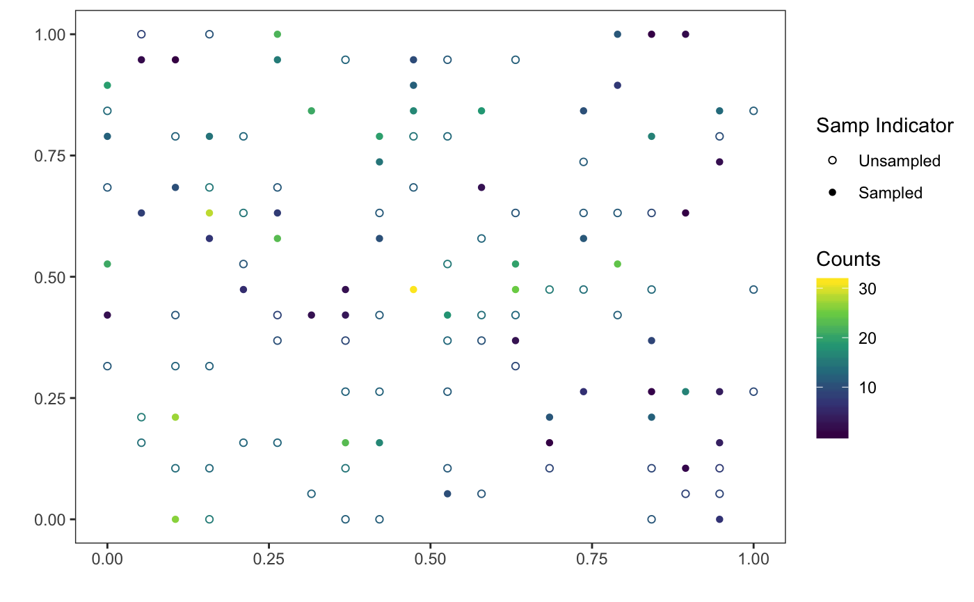
get_krigmap, get_sampdetails, get_variogram, are options to get a plot of the predictions, get some tables with details of the sampling, get a variogram of the residuals with the fitted model, and get an HTML report, respectively. These are set to FALSE by default.

outputobj <- FPBKoutput(pred_info = predobj,
  conf_level = c(0.80, 0.90, 0.95),
  get_krigmap = TRUE, get_sampdetails = TRUE,
  get_variogram = TRUE)

We can get the data set with site-by-site predictions as

pred_df <- outputobj$predvals
head(pred_df)

The column with the predictions is generally named name_of_count_variable_pred. We can get a report from the outputobj as

get_reportdoc(outputobj)

A couple of extra notes

The sites in the simulatd data set have equal area, so including area is not important or necessary. If sites have very different areas, then it is important to specify the column that has the areas in the areacol argument. Note that since all of the areas are exactly the same for the sites, we get the same prediction for the total and the same standard error whether area is included or not.

slmobj_noarea <- slmfit(formula = Moose ~ 1,
  data = highdf,
  xcoordcol = "Xcoords",
  ycoordcol = "Ycoords",
  CorModel = "Exponential",
  areacol = NULL)
predobj_noarea <- predict(object = slmobj_noarea)
predobj$FPBK_Prediction
#>          [,1]
#> [1,] 1080.689
sqrt(predobj$PredVar)
#>          [,1]
#> [1,] 81.74994
predobj_noarea$FPBK_Prediction
#>          [,1]
#> [1,] 1080.689
sqrt(predobj_noarea$PredVar)
#>          [,1]
#> [1,] 81.74994

Secondly, there is a choice of how to include stratification in the estimator. In the current WinfoNet estimator, strata are treated completely separately in the predictions. In other words, we get a prediction, covariance parameter estimates, etc. for the low stratum and a prediction, covariance parameter estimates, etc. for the high stratum. Our total prediction is simply the sum of the stratum predictions. The extra assumption that we make is that there is no cross-correlation across the strata.

The `multistrat` Function

If implementing this method, we would only need to use a single function multistrat that has all of the necessary arguments bundled together. In addition to the arguments described above, multistrat has a stratcol argument, in which the user puts the name of the column with the stratification variable. multistrat then assumes that the user wants to fit a separate covariance model for each stratum and predicts the total for the entire region of interest as well as the totals for each stratum.

multiobj <- multistrat(formula = Moose ~ 1,
  data = simdf,
  xcoordcol = "Xcoords", ycoordcol = "Ycoords",
  stratcol = "Stratum")

We then can use the get_reportdoc function to obtain a report in html:

get_reportdoc(multiobj)

We can also obtain the data frame with site-by-site predictions:

multipred_df <- multiobj$predvals
head(multipred_df)

Another choice is to include stratification as a covariate in the formula part of the linear model. The extra assumption that we would make using this method is that the spatial autocorrelation structure is similar in each of the strata but that the means of the strata are different. In the case of many of the Alaskan moose data sets, this assumption does not seem to be reasonable, as the high stratum has substantially more variability and more spatial autocorrelation than the low stratum does. However, if this seems reasonable in other data sets, the code for slmfit would be:

slmobj_cov <- slmfit(formula = Moose ~ Stratum, ## add 
  ## marchstrat as a predictor
  data = simdf, ## change the data set to have all sites
  xcoordcol = "Xcoords",
  ycoordcol = "Ycoords",
  CorModel = "Exponential",
  areacol = "Area")

Note that, for either method (fitting each stratum separately or using stratum as a covariate in the linear model), the user is able to supply more than two stratum if desired.

Section 2: Constant Detection Across Sites

If we make the assumption that detection is approximately equal across all sites in the study region, then we can input an estimate of mean detection and its standard error into predict to obtain a prediction for the population total adjusted for mean detection. The estimate of mean detection and its standard error can be obtained from a variety of methods (radiocollars, double sampling, etc.). The package performs block kriging (spatial prediction) using the observed counts and then adjusts for detection in predict, obtaining a prediction variance using the delta method.

To add arguments for this adjustment in the package, there is an argument to predict called detinfo. By default, detinfo = c(1, 0), indicating perfect detection (1) and no variability about that estimate for detection (0). Suppose that we estimate detection to be 0.7 with a standard error of 0.06. For the high stratum in the simulated data set, the code to adjust for detection in this way is:

slmobj_det <- slmfit(formula = Moose ~ 1,
  data = highdf,
  xcoordcol = "Xcoords",
  ycoordcol = "Ycoords",
  CorModel = "Exponential",
  areacol = "Area")

## add detinfo argument here
meandet <- 0.7; sedet <- 0.06
predobj_det <- predict(object = slmobj_det,
  detinfo = c(meandet, sedet))
predobj_det$FPBK_Prediction
#>          [,1]
#> [1,] 1543.841
sqrt(predobj_det$PredVar)
#>          [,1]
#> [1,] 150.5765

Note that the code for slmfit remains the same while there is one additional argument to predict. As expected, our prediction for the population total increases when we take into account imperfect detection. Additionally, imperfect detection increases our uncertainty about the prediction, so our prediction error also increases when we include imperfect detection.

To obtain an estimator for the entire region, fitting covariance models for each stratum separately, we would again use the multistrat and specify the mean and standard error for detection as an argument to multistrat.

multiobjdetection <- multistrat(formula = Moose ~ 1,
  data = simdf,
  xcoordcol = "Xcoords", ycoordcol = "Ycoords",
  stratcol = "Stratum",
  detinfo = c(0.7, 0.06))

For either case, the get_reportdoc function can still be used to obtain an html report. We can also still find the data set with site-by-site predictions.

## High Stratum only:
output_objdet <- FPBKoutput(pred_info = predobj_det)
preddf <- output_objdet$predvals
get_reportdoc(output_objdet)

## Total: both stratum
preddf_strat <- multiobjdetection$predvals
get_reportdoc(preddf_strat)

Section 3: Estimating Detection Using Logistic Regression on Radiocollar Data

For some data sets, the assumption of constant detection across sites might seem reasonable. If we do not have any habitat covariates that are strongly associated with detection in the sightability trials, then we might assume constant detection. However, for the purpose of this vignette, suppose that we would like to estimate detection using a couple of covariates, named DetPred1 and DetPred2.

Let’s first examine our sightability data set (which contains the data on the sightability trials):

pander::pander(head(vignettedetection))

X	Detected	DetPred1	DetPred2
1	1	0.836	1.223
2	0	0.6441	-1.387
3	1	0.1143	-1.281
4	0	0.6889	-0.7121
5	1	0.8233	1.349
6	1	0.8571	-1.311

In order to get detection estimates using logistic regression, we use the get_detection function within this package. The get_detection function only has three arguments:

formula, an R formula of the form response ~ pred1 + pred2 + ..., where the response is the name of the column with the sightability successes and failures, and pred1, pred2, etc. are the predictors thought to be useful for predicting detection.
data is the name of the data set with the sightability trials.
varmethod is the method used to obtain the variance of the detection estimates, either "Bootstrap" by default or "Delta".

We see that the name of the column in the vignettedetection data set with the response is called Detected. Therefore, to get the detection information needed, we can run

sightability_info <- get_detection(formula = Detected ~
    DetPred1 + DetPred2,
  data = vignettedetection,
  varmethod = "Bootstrap")

The object det_info contains the information necessary for slmfit, predict and FPBKoutput to construct the prediction for the population total, adjusted for different detection across sites. The only extra argument is needed in slmfit. The argument detectionobj is, by default set to NULL. If we add the sightability_info output as its argument and proceed with predict and FPBKoutput with no other differences, we obtain the prediction adjusted for imperfect detection.

The only other aspect of the functions to note here is that the data set in slmfit MUST have columns with the same predictors as those used in get_detection. The names of these columns must be exactly the same in both data sets. For example, if I named the willow variable DetPred1 in the sightability data set but detectionpredictor1 in the full data set, the package does not know that these are actually referring to the same variable. The data set simdf includes columns for DetPred1 and DetPred2 within the data frame:

pander::pander(head(simdf[ ,2:8]))

Xcoords	Ycoords	Moose	CountPred	DetPred1	DetPred2	Stratum
0.3158	0.3158	9	4.302	0.04218	-0.7164	Low
0.7895	0.1579	23	1.901	0.9237	1.646	Low
0.8947	0.1579	NA	2.507	0.2561	-0.09647	Low
1	0	NA	2.521	0.3524	-1.82	Low
0.9474	0.5263	0	3.693	0.06458	0.8484	Low
0.3684	0.1053	NA	3.086	0.4624	-1.195	High

So, let’s obtain a prediction for the high stratum first, adjusting for imperfect detection using logistic regression.

slmobj_dethigh <- slmfit(formula = Moose ~ 1,
  data = highdf,
  xcoordcol = "Xcoords",
  ycoordcol = "Ycoords",
  CorModel = "Exponential",
  estmethod = "ML",
  areacol = "Area",
  detectionobj = sightability_info)

predobj_dethigh <- predict(object = slmobj_dethigh)
predobj_dethigh$FPBK_Prediction
#>          [,1]
#> [1,] 1507.472
output_sightability <- FPBKoutput(pred_info = predobj_dethigh)
#>      Prediction SE(Prediction)
#> [1,]   1507.472       184.7496
#>      Lower Bound Upper Bound Proportion of Mean
#> 80 %        1271        1744               0.16
#> 90 %        1204        1811               0.20
#> 95 %        1145        1870               0.24
#>      Numb. Sites Sampled Total Numb. Sites Animals Counted Total Area
#> [1,]                  60               127             501        254
#>      Area Sampled
#> [1,]          120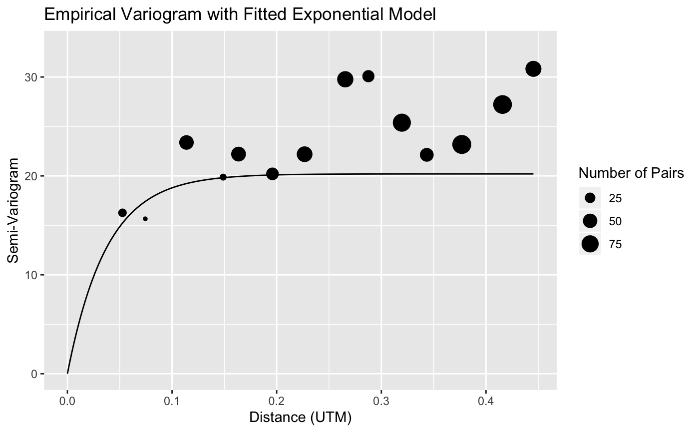

We can also predict the population total, fitting a covariance model for the high and low strata separately using multistrat:

multiobjsightability <- multistrat(formula = Moose ~ 1,
  data = simdf,
  xcoordcol = "Xcoords", ycoordcol = "Ycoords",
  stratcol = "Stratum",
  detectionobj = sightability_info)

We can obtain an html report as well as the data set with site-by-site predictions using the same functions as when we assumed perfect detection and constant detection:

get_reportdoc(output_sightability)
output_sightability$predvals

get_reportdoc(multiobjsightability)
multiobjsightability$predvals

Predicting for a Quantity Other than the Population Total

Be default, the functions within this package assume that the goal is to predict the population total across all sites in the data set specified in data. Another goal that managers might have is to predict the total in a specific section of the larger study area (for example, a game management unit). In order to predict a quantity other than the total, the user must specify the name of the column in the data set that has the desired prediction weights. A 1 or TRUE in the prediciton weight column corresponds to a site that should be included in the prediction while a 0 or FALSE corresponds to a site that should not be included in the prediction. For example, in the simdf data set, the ID numbers assigned to the 400 sites are 1 through 400. These ID numbers are given in column X of the data set. Suppose that I just want to predict the population total for sites 1 through 100. Then, I could define a new column in the data set as

simdf$predwts <- as.numeric(simdf$X <= 100)
pander::pander(simdf[1:7, c("X", "Moose", "predwts")])

X	Moose	predwts
127	9	0
76	23	1
78	NA	1
20	NA	1
219	0	0
48	NA	1
96	NA	1

Notice how any site with an ID number less than or equal to 100 has a 1 in the predwts column.

Then, in the predict function, I would include the FPBKcol argument and give the name of the column with the prediction weights. In the example below, stratum is included as a covariate in the linear model.

slmobj_predwts <- slmfit(formula = Moose ~ Stratum,
  data = simdf,
  xcoordcol = "Xcoords",
  ycoordcol = "Ycoords",
  CorModel = "Exponential",
  estmethod = "ML",
  areacol = "Area",
  detectionobj = sightability_info)
predobj_predwts <- predict(object = slmobj_predwts,
  FPBKcol = "predwts") ## added FPBKcol argument here
predobj_predwts$FPBK_Prediction
#>          [,1]
#> [1,] 1730.906
sqrt(predobj_predwts$PredVar)
#>         [,1]
#> [1,] 209.954
output_predwts <- FPBKoutput(predobj_predwts)
#>      Prediction SE(Prediction)
#> [1,]   1730.906        209.954
#>      Lower Bound Upper Bound Proportion of Mean
#> 80 %        1462        2000               0.16
#> 90 %        1386        2076               0.20
#> 95 %        1319        2142               0.24
#>      Numb. Sites Sampled Total Numb. Sites Animals Counted Total Area
#> [1,]                 100               400            1011        800
#>      Area Sampled
#> [1,]          200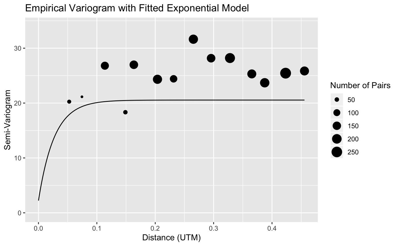

If fitting a separate covariance model for each stratum, we would incorporate the FPBKcol argument in the multistrat function:

multiobj_predwts <- multistrat(formula = Moose ~ 1,
  data = simdf,
  xcoordcol = "Xcoords", ycoordcol = "Ycoords",
  stratcol = "Stratum",
  detectionobj = sightability_info,
  FPBKcol = "predwts")

The resulting prediction and standard error are then associated with the region of interest. We can again obtain a data frame with site-by-site predictions as well as an html report specifying the $predvals output to multiobj_predwts or output_predwts and using the get_reportdoc function.

Conclusion

We have used the FPBKPack2 to predict the moose population total in the Togiak National Wildlife Refuge with the four main functions slmfit, predict, FPBKoutput, and multistrat. Both the structure of the data needed to be input into the functions and the output report constructed from using the functions are meant to be similar to the WinfoNet input and output.

(Link to Github Page)

Matt Higham

2019-09-08

Introduction

Section 1: Perfect Detection

R Shiny App

Package Functions

The `slmfit` Function

The `predict` Function

The `FPBKoutput` Function

A couple of extra notes

The `multistrat` Function

Section 2: Constant Detection Across Sites

Section 3: Estimating Detection Using Logistic Regression on Radiocollar Data

Predicting for a Quantity Other than the Population Total

Conclusion

Contents

Using the GSPE R Package

Matt Higham

2019-09-08

Introduction

Section 1: Perfect Detection

R Shiny App

Package Functions

The slmfit Function

The predict Function

The FPBKoutput Function

A couple of extra notes

The multistrat Function

Section 2: Constant Detection Across Sites

Section 3: Estimating Detection Using Logistic Regression on Radiocollar Data

Predicting for a Quantity Other than the Population Total

Conclusion

Contents

The `slmfit` Function

The `predict` Function

The `FPBKoutput` Function

The `multistrat` Function